Visualizing Audio for Anomaly Detection Mark HasegawaJohnson Camille

Research Goal: Guide audio analysts to anomalies • Large dataset: audio • Anomalies •

• Feature : audio interval numbers • Visualization : numbers rendering • Audio-based

Audio-Based Features: Transformed acoustic data • Pitch, Formants • Anomaly Salience Score • Waveform

Model-Based Features • • Log-likelihood features Display how well a hypothesis fits Let analyst

Model-Based Features • Log-likelihood features Log-likelihood ratios (LLR) • Because Mixture Gaussian misclassifies outliers

Too many features! • Evaluate each feature with Kullback-Leibler Divergence • Combine features with

Two Interactive Testbeds • • • Vary features Vary anomalies Vary background audio Vary

Human Subject Protocols • Tutorial • Training with immediate feedback • Measure how fast

Influence on FODAVA • Guide, don’t replace, human analysts • Guide them with zoomable

Developing FODAVA • Make “big” audio accessible • Audio is hard, but its concepts

Slides: 16

Download presentation

Visualizing Audio for Anomaly Detection Mark Hasegawa-Johnson Camille Goudeseune Hank Kaczmarski Thomas Huang University of Illinois at Urbana-Champaign

Research Goal: Guide audio analysts to anomalies • Large dataset: audio • Anomalies • Cheap to record, expensive to play • GUI: listen 10000 x faster • Robots are poor listeners, but good servants

• Anomalies shoot down poor theories

• Feature : audio interval numbers • Visualization : numbers rendering • Audio-based features (spectrogram) • Model-based features (Hnull, Hthreatening)

Audio-Based Features: Transformed acoustic data • Pitch, Formants • Anomaly Salience Score • Waveform A = f(t) • Spectrogram A = f(t, Hz) • Correlogram A = f(t, Hz, fundamental period) • Rate-scale representation A = f(t, Hz, bandwidth, ΔHz) • Wavelets • Multiscale

Model-Based Features • • Log-likelihood features Display how well a hypothesis fits Let analyst intuit a threshold of fitness Defined by Mixture Gaussians, trained by: EM Parzen Windows One-class SVMs

Model-Based Features • Log-likelihood features Log-likelihood ratios (LLR) • Because Mixture Gaussian misclassifies outliers as anomalies

Too many features! • Evaluate each feature with Kullback-Leibler Divergence • Combine features with Ada. Boost + SVM + HMM

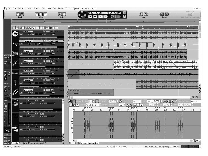
Two Interactive Testbeds • • • Vary features Vary anomalies Vary background audio Vary how model is trained Vary mapping from features to HSV • Anomalousness “bubbles up”

Multi-day audio timeline

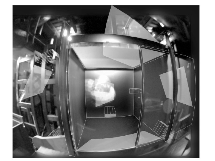
1000 μphone = The Milliphone

Human Subject Protocols • Tutorial • Training with immediate feedback • Measure how fast subjects find x% of anomalies

Influence on FODAVA • Guide, don’t replace, human analysts • Guide them with zoomable features • Features from transformed data (audio-based) • Features from fitting hypotheses (model-based)

Developing FODAVA • Make “big” audio accessible • Audio is hard, but its concepts generalize • Fast interactive exploration of time series, long (timeline) or wide (milliphone)