Visualization of the hidden node activities or hidden

Visualization of the hidden node activities or hidden secrets of neural networks. Włodzisław Duch Department of Informatics Nicolaus Copernicus University, Toruń, Poland School of Computer Engineering, Nanyang Technological University, Singapore Google: Duch ICAISC Zakopane June 2004

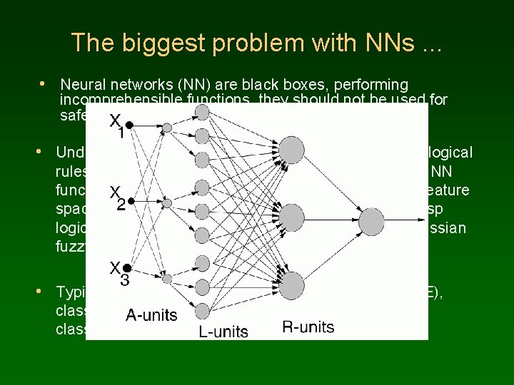
The biggest problem with NNs. . . • Neural networks (NN) are black boxes, performing incomprehensible functions, they should not be used for safety-critical applications. • Understanding of network decisions is possible using logical rules (Duch et al 2001), but logical rules equivalent to NN functions severely distort original decision borders. Feature space is partitioned by rules into hypercuboids (for crisp logical rules) or ellipsoids (for typical triangular or Gaussian fuzzy membership functions). • Typical NN software outputs: mean square error (MSE), classification error, sometimes estimation of the classification probability, rarely ROC curves.

NNs dangers. . . • But: perhaps errors are confined to a distant and localized region of the feature space? How to estimate confidence in predictions, distinguish easy/difficult cases? • Well trained MLPs provide estimations of p(C|X) close to 0 • • • and 1: they are overconfident in their predictions. 10 errors with p(C|X) 1 are more dangerous than 20 with p(C|X) 0. 5. How to compare networks that have identical accuracy, but quite different weights and biases? Is the network hiding a quirky behavior that may lead to completely wrong results for new data? Is regularization improving the quality of NN? If I only could see it. . . but how? Feature spaces are high D. Look at mapping of the training data samples, their similarities! K nodes => scatterograms in K-dimensional space.

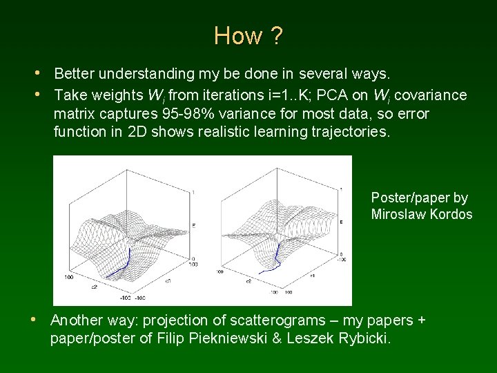
How ? • Better understanding my be done in several ways. • Take weights Wi from iterations i=1. . K; PCA on Wi covariance matrix captures 95 -98% variance for most data, so error function in 2 D shows realistic learning trajectories. Poster/paper by Miroslaw Kordos • Another way: projection of scatterograms – my papers + paper/poster of Filip Piekniewski & Leszek Rybicki.

What feedforward NN really do? Vector mappings from the input space to hidden space(s) and to the output space. Hidden-Output mapping done by perceptrons. A single hidden layer case is analyzed below. T = {Xi} H = {hj(Xi)} training data, N-dimensional. T image in the hidden space, j =1. . NH-dim. Y = {yk{h(Xi)} T image in the output space, k =1. . NC-dim. ANN goal: scatterograms of T in the hidden space should be linearly separable; internal representations will determine network generalization capabilities and other properties.

What can we see? Output images of the training data vectors mapped by NN: • show the dynamics of learning, problems with convergence; • show overfitting and underfitting effects; • enable to compare different network solution with the same • • MSE/accuracy, compare training algorithms, inspect classification margins perturbing the input vectors; display regions of the input space where potential problems may arise; show stability of network classification under perturbation of original vectors; display effects of regularization, model selection, early stopping; enable quick identification of errors and outliers; estimate confidence in classification of a given vector by placing it in relation to known data vectors. . . . .

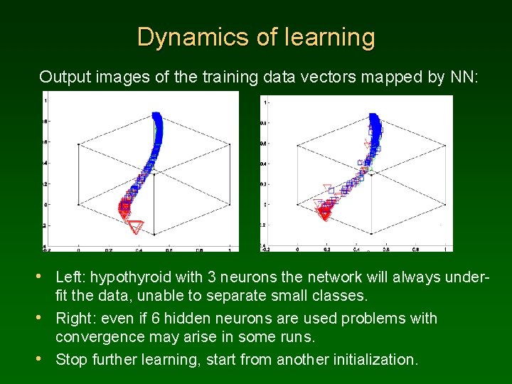
Dynamics of learning Output images of the training data vectors mapped by NN: • Left: hypothyroid with 3 neurons the network will always underfit the data, unable to separate small classes. • Right: even if 6 hidden neurons are used problems with convergence may arise in some runs. • Stop further learning, start from another initialization.

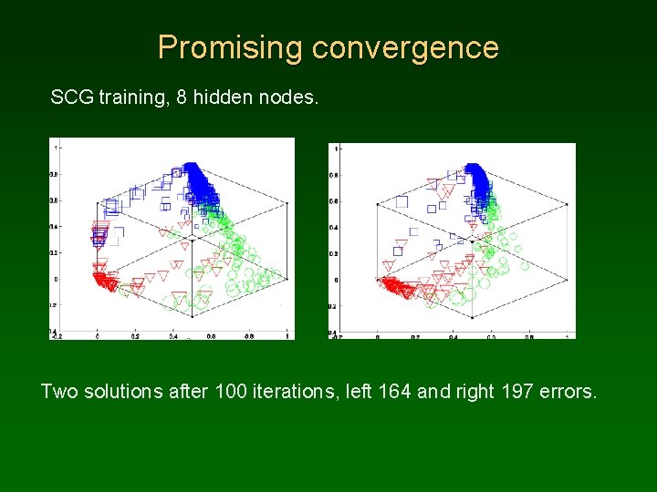
Promising convergence SCG training, 8 hidden nodes. Two solutions after 100 iterations, left 164 and right 197 errors.

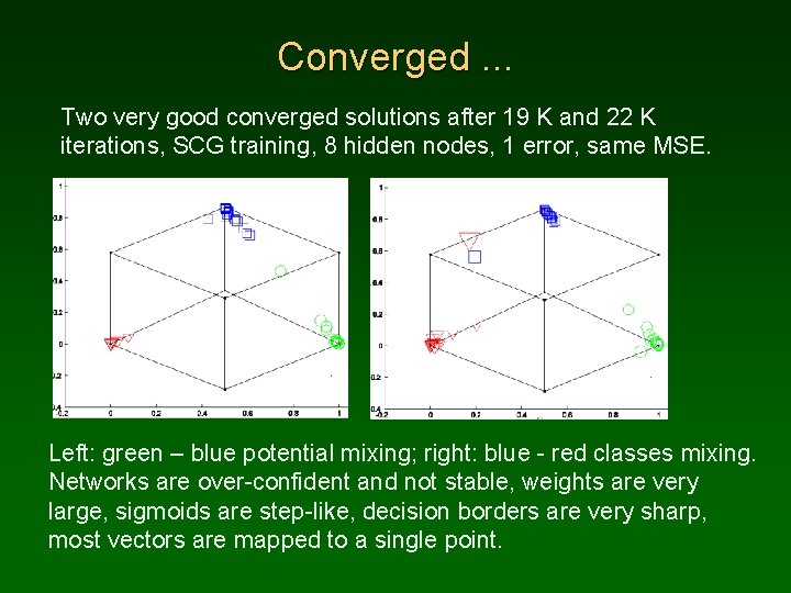
Converged. . . Two very good converged solutions after 19 K and 22 K iterations, SCG training, 8 hidden nodes, 1 error, same MSE. Left: green – blue potential mixing; right: blue - red classes mixing. Networks are over-confident and not stable, weights are very large, sigmoids are step-like, decision borders are very sharp, most vectors are mapped to a single point.

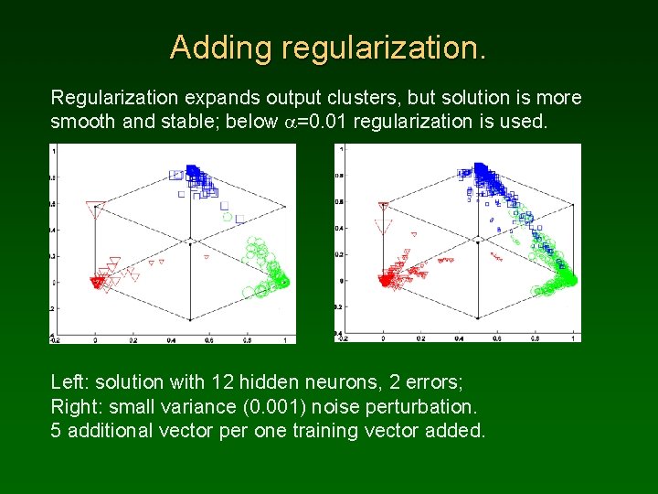
Adding regularization. Regularization expands output clusters, but solution is more smooth and stable; below a=0. 01 regularization is used. Left: solution with 12 hidden neurons, 2 errors; Right: small variance (0. 001) noise perturbation. 5 additional vector per one training vector added.

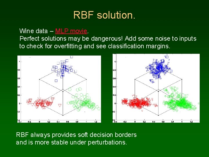
RBF solution. Wine data – MLP movie. Perfect solutions may be dangerous! Add some noise to inputs to check for overfitting and see classification margins. RBF always provides soft decision borders and is more stable under perturbations.

What is inside? Many types of internal representations may look identical from outside, but generalization may depend on them. • Classify different types of internal representations. • Take permutational invariance into account: equivalent • • • internal representations may be obtained by re-numbering hidden nodes. Good internal representations should form compact clusters in the internal space. Check if the representations form separable clusters. Discover poor representations and stop training. Analyze adaptive capacity of networks. . .

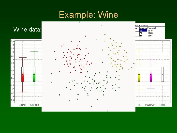
Example: Wine data:

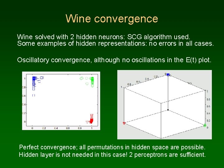
Wine convergence Wine solved with 2 hidden neurons: SCG algorithm used. Some examples of hidden representations: no errors in all cases. Oscillatory convergence, although no oscillations in the E(t) plot. Perfect convergence; all permutations in hidden space are possible. Hidden layer is not needed in this case! 2 perceptrons are sufficient.

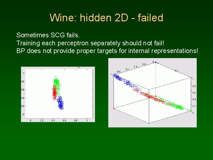
Wine: hidden 2 D - failed Sometimes SCG fails. Training each perceptron separately should not fail! BP does not provide proper targets for internal representations!

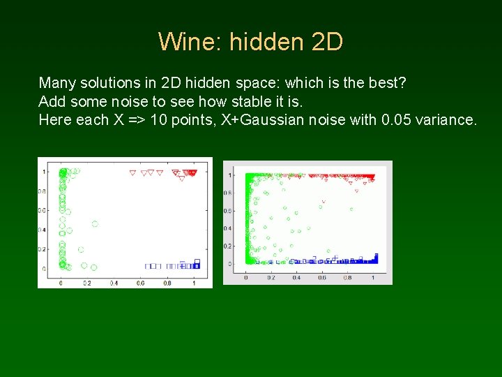
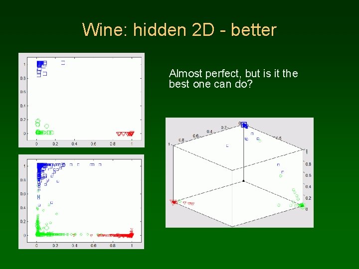
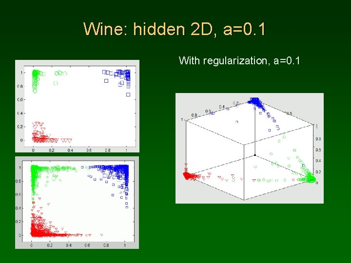
Wine: hidden 2 D Many solutions in 2 D hidden space: which is the best? Add some noise to see how stable it is. Here each X => 10 points, X+Gaussian noise with 0. 05 variance.

Wine: hidden 2 D - better Almost perfect, but is it the best one can do?

Wine: hidden 2 D, a=0. 1 With regularization, a=0. 1

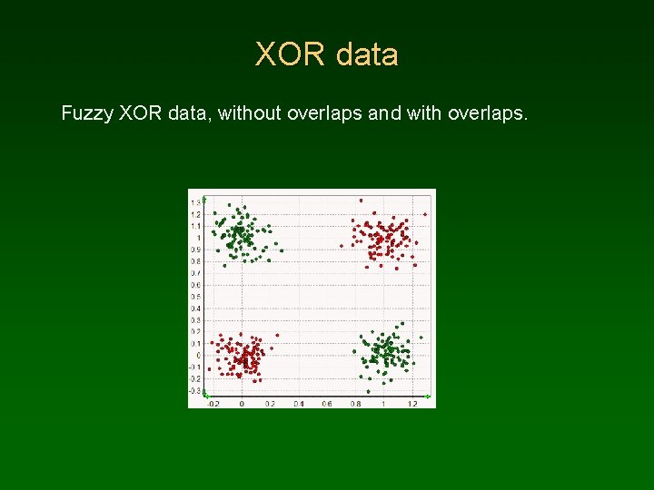
XOR data Fuzzy XOR data, without overlaps and with overlaps.

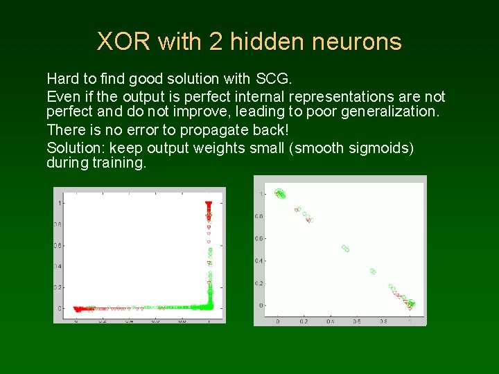
XOR with 2 hidden neurons Hard to find good solution with SCG. Even if the output is perfect internal representations are not perfect and do not improve, leading to poor generalization. There is no error to propagate back! Solution: keep output weights small (smooth sigmoids) during training.

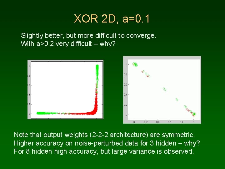
XOR 2 D, a=0. 1 Slightly better, but more difficult to converge. With a>0. 2 very difficult – why? Note that output weights (2 -2 -2 architecture) are symmetric. Higher accuracy on noise-perturbed data for 3 hidden – why? For 8 hidden high accuracy, but large variance is observed.

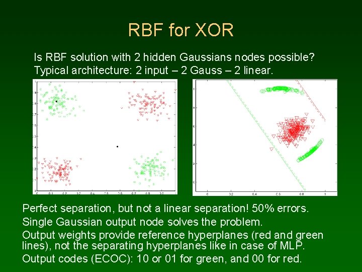
RBF for XOR Is RBF solution with 2 hidden Gaussians nodes possible? Typical architecture: 2 input – 2 Gauss – 2 linear. Perfect separation, but not a linear separation! 50% errors. Single Gaussian output node solves the problem. Output weights provide reference hyperplanes (red and green lines), not the separating hyperplanes like in case of MLP. Output codes (ECOC): 10 or 01 for green, and 00 for red.

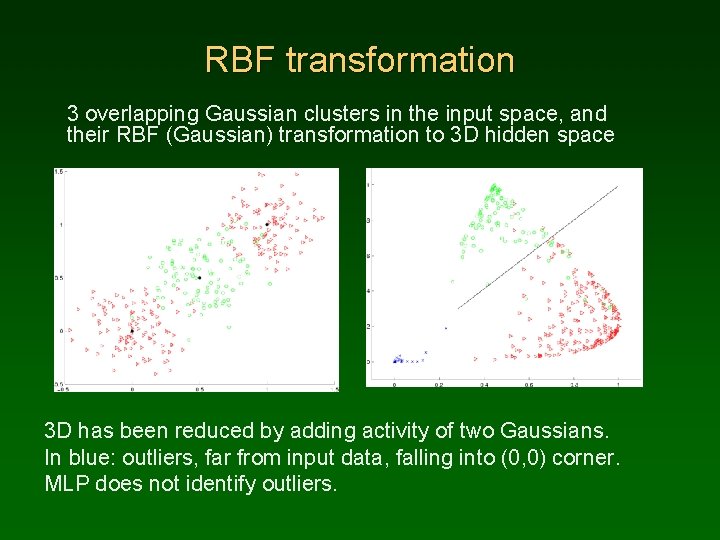
RBF transformation 3 overlapping Gaussian clusters in the input space, and their RBF (Gaussian) transformation to 3 D hidden space 3 D has been reduced by adding activity of two Gaussians. In blue: outliers, far from input data, falling into (0, 0) corner. MLP does not identify outliers.

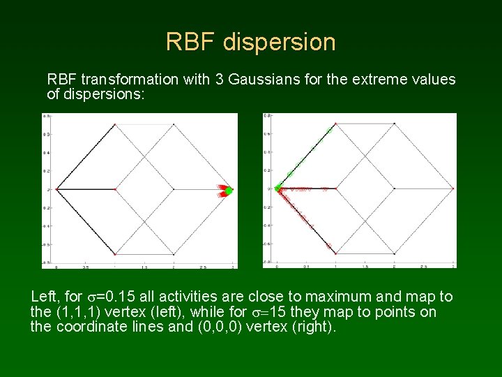
RBF dispersion RBF transformation with 3 Gaussians for the extreme values of dispersions: Left, for s=0. 15 all activities are close to maximum and map to the (1, 1, 1) vertex (left), while for s=15 they map to points on the coordinate lines and (0, 0, 0) vertex (right).

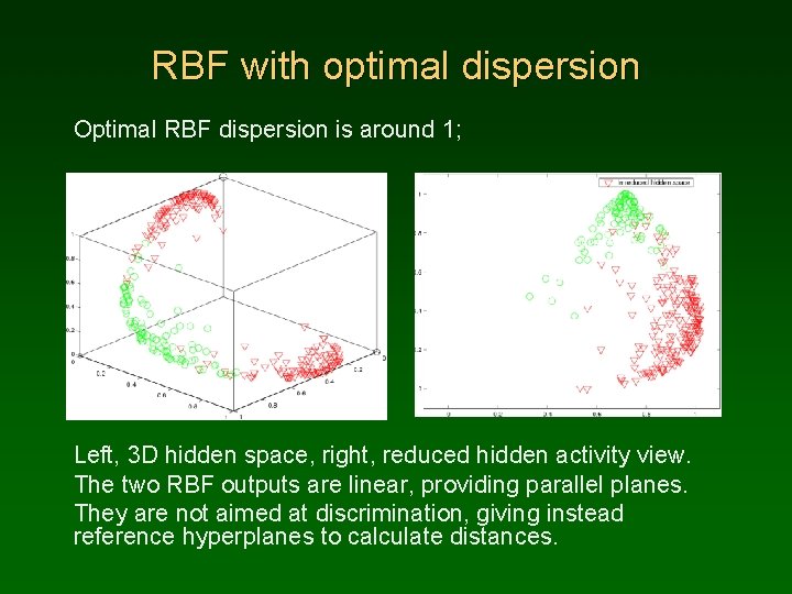
RBF with optimal dispersion Optimal RBF dispersion is around 1; Left, 3 D hidden space, right, reduced hidden activity view. The two RBF outputs are linear, providing parallel planes. They are not aimed at discrimination, giving instead reference hyperplanes to calculate distances.

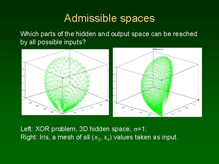
Admissible spaces Which parts of the hidden and output space can be reached by all possible inputs? Left: XOR problem, 3 D hidden space, s=1; Right: Iris, a mesh of all (x 3, x 4) values taken as input.

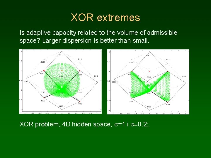
XOR extremes Is adaptive capacity related to the volume of admissible space? Larger dispersion is better than small. XOR problem, 4 D hidden space, s=1 i s=0. 2;

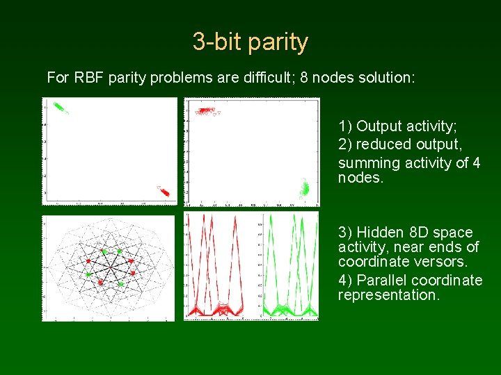
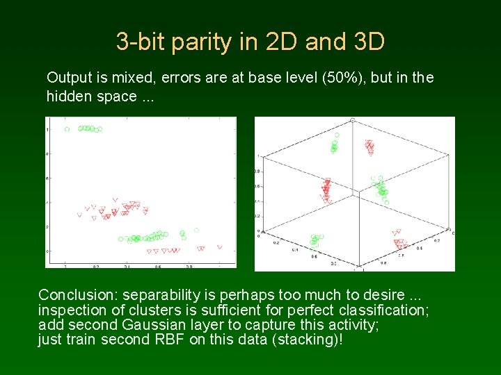
3 -bit parity For RBF parity problems are difficult; 8 nodes solution: 1) Output activity; 2) reduced output, summing activity of 4 nodes. 3) Hidden 8 D space activity, near ends of coordinate versors. 4) Parallel coordinate representation.

3 -bit parity in 2 D and 3 D Output is mixed, errors are at base level (50%), but in the hidden space. . . Conclusion: separability is perhaps too much to desire. . . inspection of clusters is sufficient for perfect classification; add second Gaussian layer to capture this activity; just train second RBF on this data (stacking)!

Thank you for lending your ears. . .