Visual DSD a design and analysis tool for

Visual DSD: a design and analysis tool for DNA strand displacement systems Matthew R. Lakin, Simon Youssef, Filippo Polo, Stephen Emmott and Andrew Phillips Microsoft Research, Cambridge (ppt by John Reif) Matthew R. Lakin, Simon Youssef, Filippo Polo, Stephen Emmott, and Andrew Phillips, Visual DSD: a design and analysis tool for DNA strand displacement systems, Bioinformatics. 2011 Nov 15; 27(22): 3211– 3213. http: //www. ncbi. nlm. nih. gov/pmc/articles/PMC 3208393/ Matthew R. Lakin David Parker, Luca Cardelli, Marta Kwiatkowska and Andrew Phillips, Design and analysis of DNA strand displacement devices using probabilistic model checking, J. R. Soc. Interface. doi: 10. 1098/rsif. 2011. 0800 http: //rsif. royalsocietypublishing. org/content/early/2012/01/03/rsif. 2011. 0800

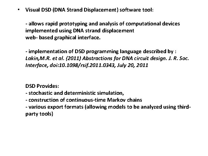
• Visual DSD (DNA Strand Displacement) software tool: - allows rapid prototyping and analysis of computational devices implemented using DNA strand displacement web- based graphical interface. - implementation of DSD programming language described by : Lakin, M. R. et al. (2011) Abstractions for DNA circuit design. J. R. Soc. Interface, doi: 10. 1098/rsif. 2011. 0343, July 20, 2011 DSD Provides: - stochastic and deterministic simulation, - construction of continuous-time Markov chains - various export formats (allowing models to be analyzed using thirdparty tools)

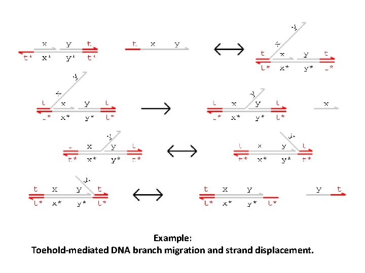
Example: Toehold-mediated DNA branch migration and strand displacement.

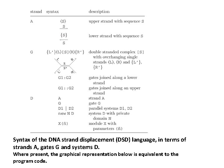
Syntax of the DNA strand displacement (DSD) language, in terms of strands A, gates G and systems D. Where present, the graphical representation below is equivalent to the program code.

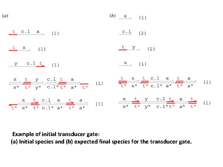
Example of initial transducer gate: (a) Initial species and (b) expected final species for the transducer gate.

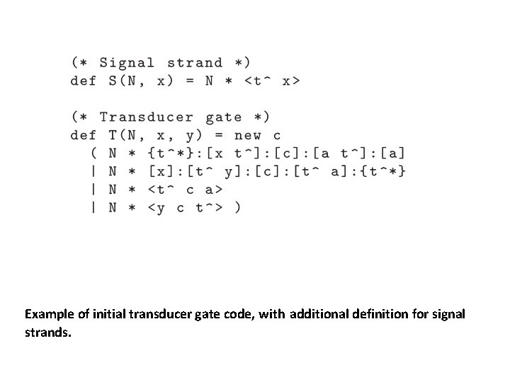
Example of initial transducer gate code, with additional definition for signal strands.

Model Checking Is an automated formal verification technique, based on the exhaustive construction and analysis of a finite-state model of the system being verified. - The model is usually a labelled state-transition system, in which each state represents a possible configuration of the system and each transition between states represents a possible evolution from one configuration to another. - The desired correctness properties of the system are typically expressed in temporal logics, such as computation tree logic (CTL) or linear-time temporal logic. Example typical CTL formulae (along with their corresponding informal meanings): — A [ G !(“access 1” & “access 2”): ‘processes 1 and 2 never simultaneously access a shared resource’ — A [ F “end” ]: ‘the algorithm always eventually terminates’ — E [ !“fail” U “end” ]: ‘it is possible for the algorithm to terminate without any failures occurring’. Model Checker: - Once the desired correctness properties of the system have been formally expressed in this way, they can then be verified using a model checker. - This performs an exhaustive analysis of the system model, for each property either concluding that it is satisfied or, if not, providing a counterexample illustrating why it is violated.

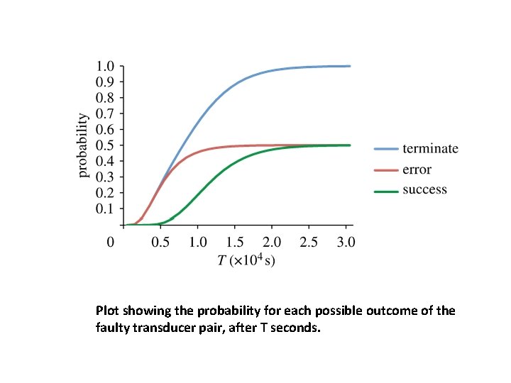
Probabilistic model checking This is a generalization of model checking for the verification of systems that exhibit stochastic behaviour. - The models that are constructed analysed are augmented with quantitative information regarding the likelihood that transitions occur and the times at which they do so. - In practice, these models are typically Markov chains or Markov decision processes. To model systems of reactions at a molecular level, the appropriate model is continuous-time Markov chains (CTMCs), in which transitions between states are assigned (positive, real- valued) rates. These values are interpreted as the rates of negative exponential distributions. Properties of CTMCs are, like in non-probabilistic model checking, expressed in temporal logic, but are now expressed quantitative in nature. - For this, one uses probabilistic temporal logics such as continuous stochastic logic (CSL. - For example: rather than verifying that ‘the protein always eventually degrades’, using CSL allows us to ask ‘what is the probability that the protein eventually degrades? ’ or ‘what is the probability that the protein degrades within t hours? ’

Plot showing the probability for each possible outcome of the faulty transducer pair, after T seconds.

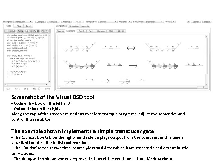
Screenshot of the Visual DSD tool: - Code entry box on the left and - Output tabs on the right. Along the top of the screen are options to select example programs, adjust the semantics and control the simulator. The example shown implements a simple transducer gate: - The Compilation tab on the right-hand side displays output from the compiler, in this case a visualization of all the individual reactions. - The Simulation tab shows time-course plots and data tables from stochastic and deterministic simulations. - The Analysis tab shows various representations of the continuous-time Markov chain.

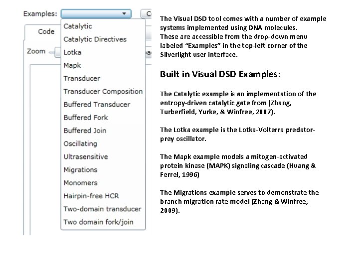
The Visual DSD tool comes with a number of example systems implemented using DNA molecules. These are accessible from the drop-down menu labeled “Examples” in the top-left corner of the Silverlight user interface. Built in Visual DSD Examples: The Catalytic example is an implementation of the entropy-driven catalytic gate from (Zhang, Turberfield, Yurke, & Winfree, 2007). The Lotka example is the Lotka-Volterra predatorprey oscillator. The Mapk example models a mitogen-activated protein kinase (MAPK) signaling cascade (Huang & Ferrel, 1996) The Migrations example serves to demonstrate the branch migration rate model (Zhang & Winfree, 2009).

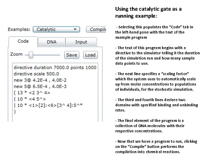
Using the catalytic gate as a running example: - Selecting this populates the “Code” tab in the left-hand pane with the text of the example program - The text of this program begins with a directive to the simulator telling it the duration of the simulation run and how many sample data points to use. - The next line specifies a “scaling factor” which the system uses to automatically scale up from molar concentrations to populations of individuals, for the stochastic simulation. - The third and fourth lines declare two domains with specified binding and unbinding rates. - The final element of the program is a collection of DNA molecules with their respective concentrations. - Now that we have a program to run, clicking on the “Compile” button performs the compilation into chemical reactions.

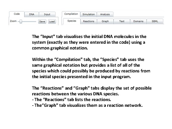
The “Input” tab visualises the initial DNA molecules in the system (exactly as they were entered in the code) using a common graphical notation. Within the “Compilation” tab, the “Species” tab uses the same graphical notation but provides a list of all of the species which could possibly be produced by reactions from the initial species presented in the input program. The “Reactions” and “Graph” tabs display the set of possible reactions between the various DNA species. - The “Reactions” tab lists the reactions. - The“Graph” tab visualizes them as a reaction network.

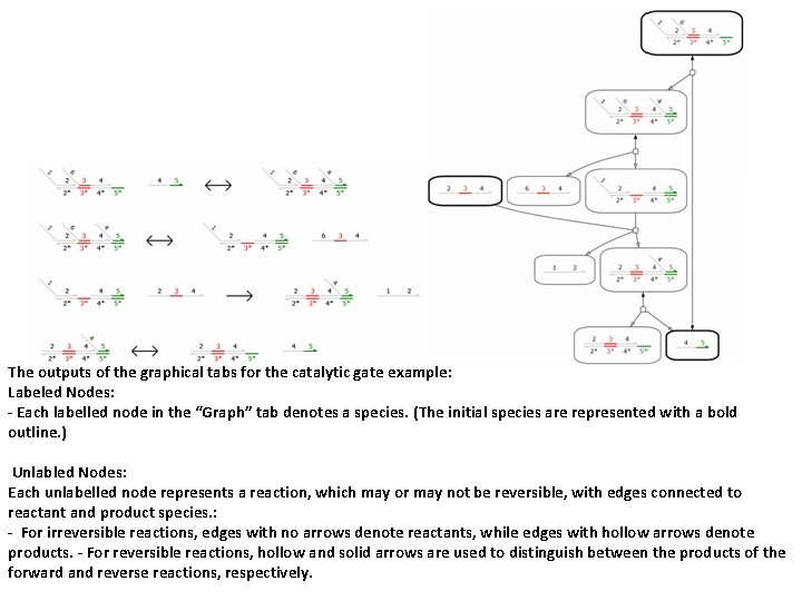
The outputs of the graphical tabs for the catalytic gate example: Labeled Nodes: - Each labelled node in the “Graph” tab denotes a species. (The initial species are represented with a bold outline. ) Unlabled Nodes: Each unlabelled node represents a reaction, which may or may not be reversible, with edges connected to reactant and product species. : - For irreversible reactions, edges with no arrows denote reactants, while edges with hollow arrows denote products. - For reversible reactions, hollow and solid arrows are used to distinguish between the products of the forward and reverse reactions, respectively.

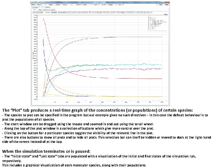
The “Plot” tab produces a real-time graph of the concentrations (or populations) of certain species: - The species to plot can be specified in the program but our example gives no such directives – in this case the default behaviour is to plot the populations of all species. - The chart window can be dragged using the mouse and zoomed in and out using the scroll wheel. - Along the top of the plot window is a collection of buttons which give more control over the plot. - Clicking on the button for a particular species toggles the visibility of the relevant line in the plot. - There also buttons to show all plots and to hide all plots. This selection bar can itself be hidden or moved to dock at the right-hand side of the screen instead of at the top. When the simulation terminates or is paused: - The “Initial state” and “Last state” tabs are populated with a visualization of the initial and final states of the simulation run, respectively. This includes a graphical visualization of each molecular species, along with their populations.