Visibility Graph Voronoi Diagram Control is easy stay
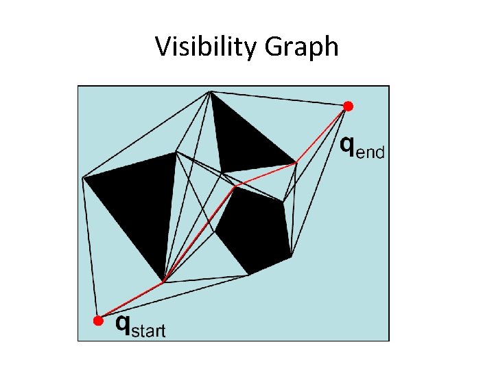
Visibility Graph
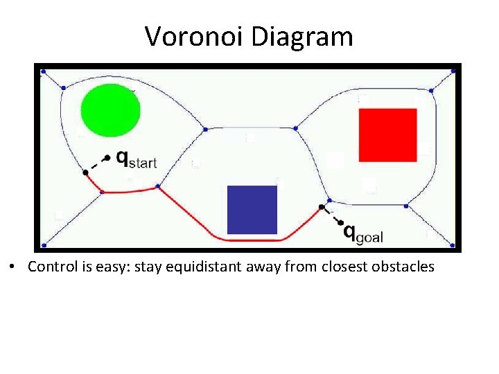
Voronoi Diagram • Control is easy: stay equidistant away from closest obstacles
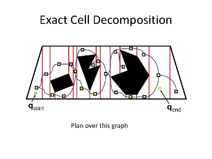
Exact Cell Decomposition Plan over this graph
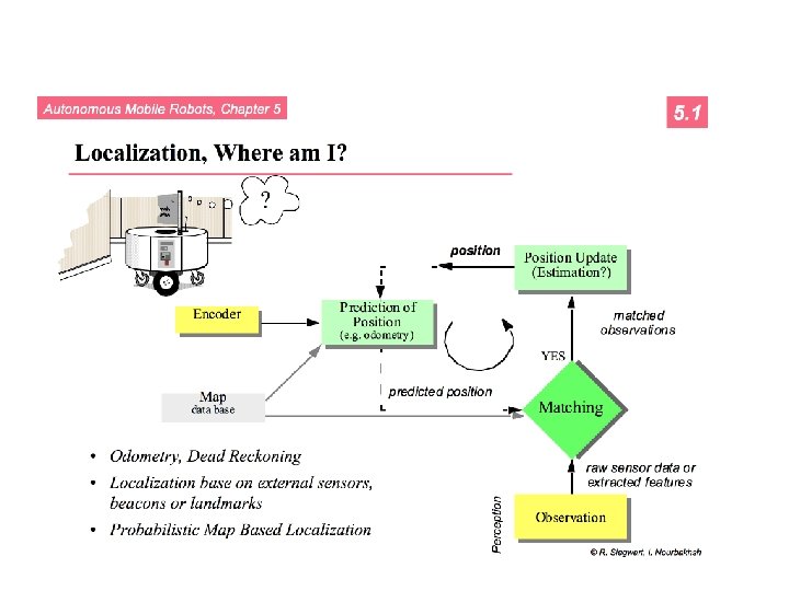
Localization • Two types of approaches: – Iconic : use raw sensor data directly. Match current sensor readings with what was observed in the past – Feature-based : extract features of the environment, such as corners and doorways. Match current observations
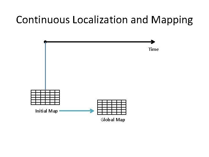
Continuous Localization and Mapping Time Initial Map Global Map
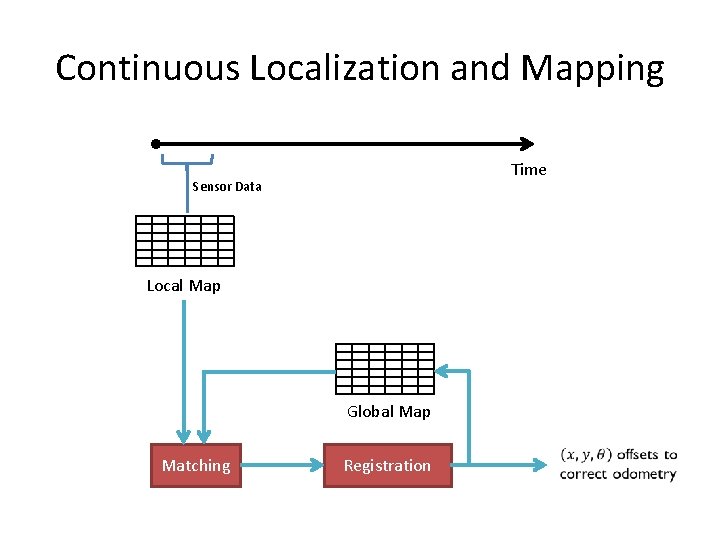
Continuous Localization and Mapping Time Sensor Data Local Map Global Map Matching Registration
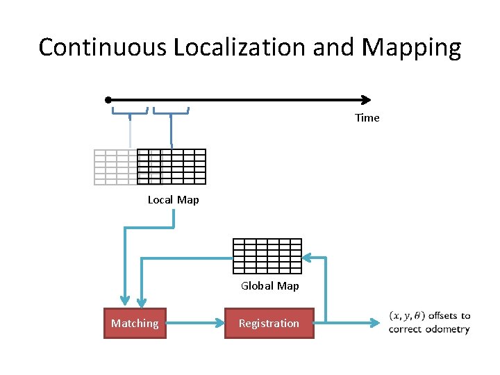
Continuous Localization and Mapping Time Local Map Global Map Matching Registration
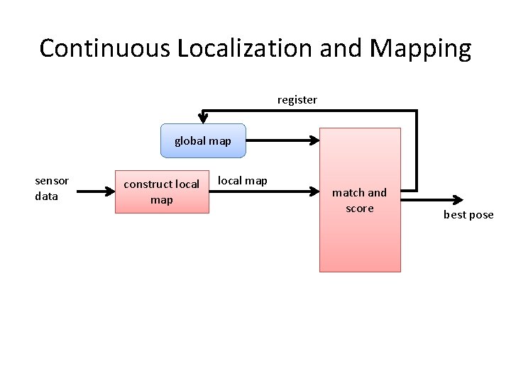
Continuous Localization and Mapping register global map sensor data construct local map match and score best pose
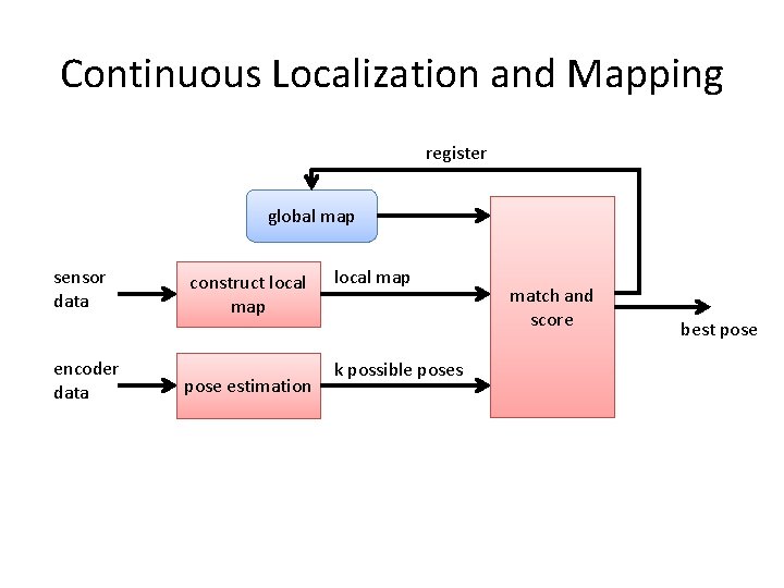
Continuous Localization and Mapping register global map sensor data encoder data construct local map pose estimation local map k possible poses match and score best pose
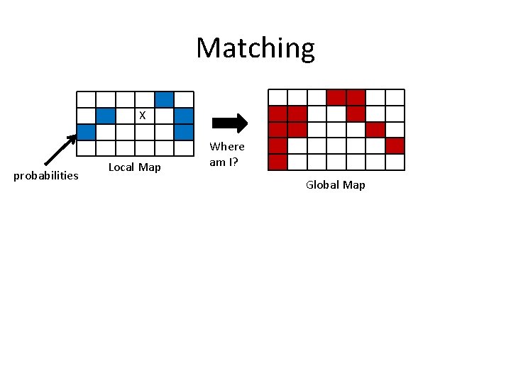
Matching X probabilities Local Map Where am I? Global Map
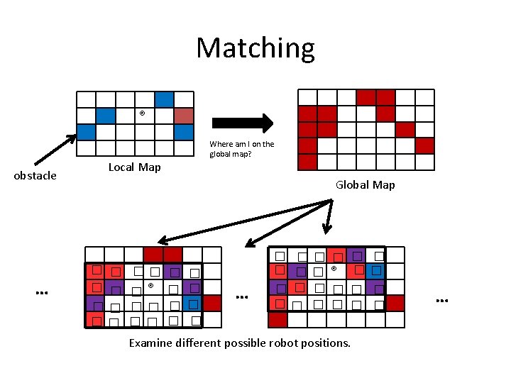
Matching ® obstacle … Where am I on the global map? Local Map Global Map � � � �® �� �� � � � � … � �� � � ® �� � � � Examine different possible robot positions. …

This sounds hard, do we need to localize? https: //www. youtube. com/watch? v=6 KRjuu. EVEZs
Matching and Registration • Collect sensor readings and create a local map • Estimate poses that the robot is likely to be in given distance traveled from last map update – In theory k is infinite – Discretize the space of possible positions (e. g. , consider errors in increments of 5 o) – Try to model the likely behavior of your robot. Try to account for systematic errors (e. g. , robot tends to drift to one side)

Matching and Registration • What if you were tracking multiple possible poses. How would you combine info from this with previous estimate of global position + odometry?
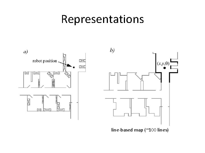
Representations line-based map (~100 lines)
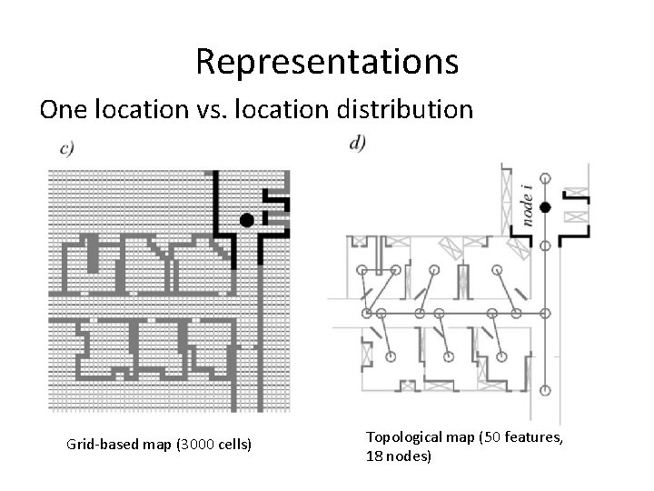
Representations One location vs. location distribution Grid-based map (3000 cells) Topological map (50 features, 18 nodes)
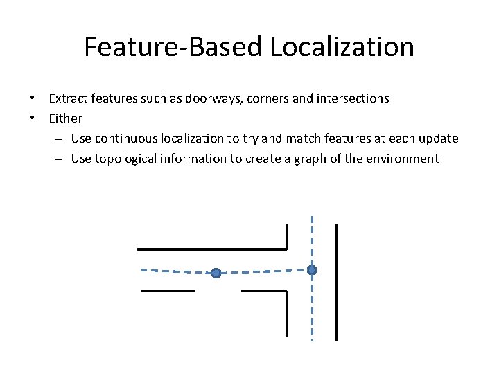
Feature-Based Localization • Extract features such as doorways, corners and intersections • Either – Use continuous localization to try and match features at each update – Use topological information to create a graph of the environment
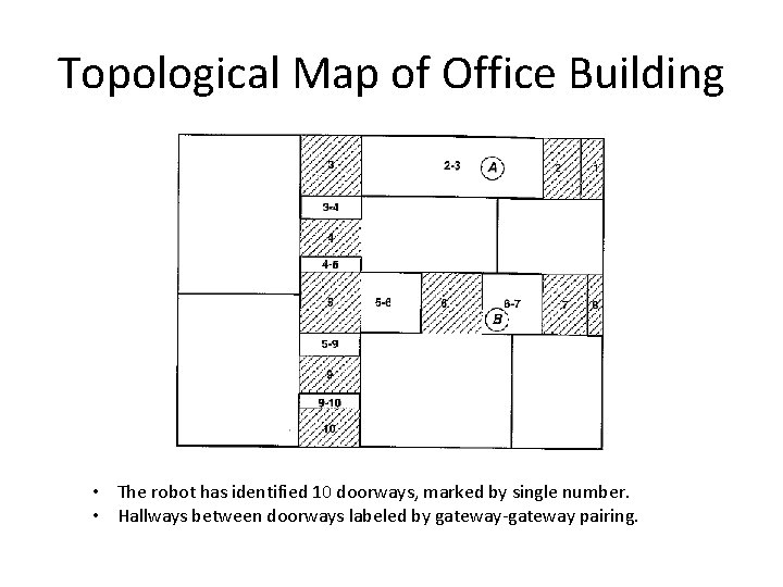
Topological Map of Office Building • The robot has identified 10 doorways, marked by single number. • Hallways between doorways labeled by gateway-gateway pairing.
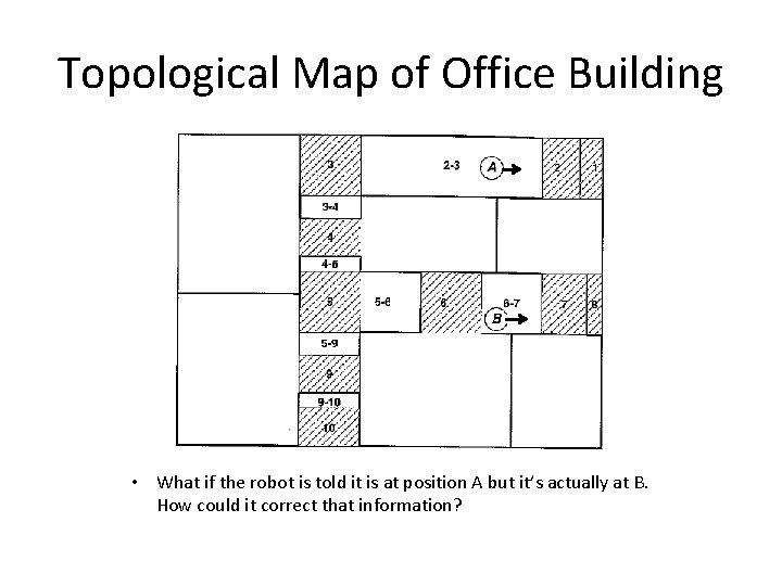
Topological Map of Office Building • What if the robot is told it is at position A but it’s actually at B. How could it correct that information?
Localization Problem(s) • • Position Tracking Global Localization Kidnapped Robot Problem Multi-Robot Localization
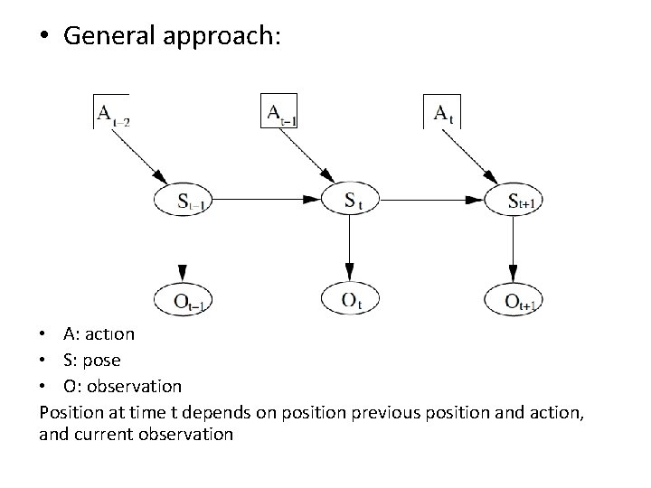
• General approach: • A: action • S: pose • O: observation Position at time t depends on position previous position and action, and current observation
• Pose at time t determines the observation at time t • If we know the pose, we can say what the observation is • But, this is backwards… • Hello Bayes!
Quiz! • If events a and b are independent, • p(a, b) = • If events a and b are not independent, • p(a, b) = • p(c|d) = ? Mattel 1992
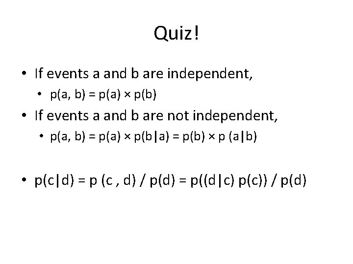
Quiz! • If events a and b are independent, • p(a, b) = p(a) × p(b) • If events a and b are not independent, • p(a, b) = p(a) × p(b|a) = p(b) × p (a|b) • p(c|d) = p (c , d) / p(d) = p((d|c) p(c)) / p(d)
Bayes Filtering • Want to have a way of representing uncertainty • Probability Distribution – Could be discrete or continuous – Prob. of each pose in set of all possible poses • Belief • Prior • Posterior
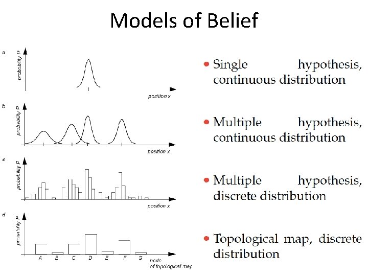
Models of Belief
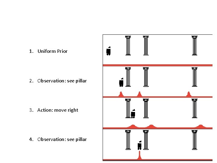
1. Uniform Prior 2. Observation: see pillar 3. Action: move right 4. Observation: see pillar
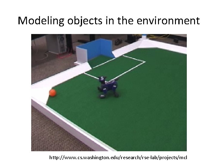
Modeling objects in the environment http: //www. cs. washington. edu/research/rse-lab/projects/mcl
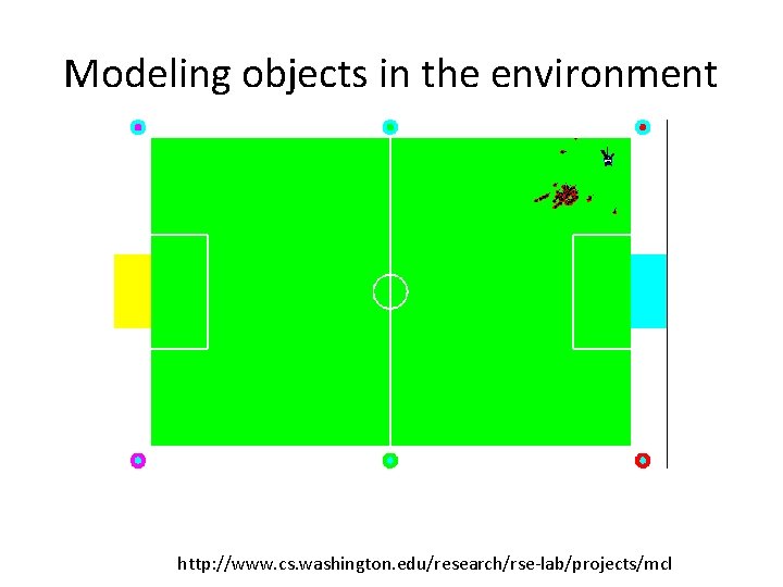
Modeling objects in the environment http: //www. cs. washington. edu/research/rse-lab/projects/mcl
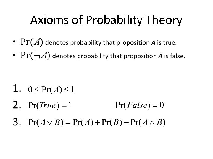
Axioms of Probability Theory •
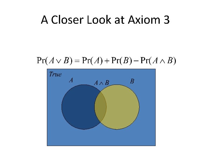
A Closer Look at Axiom 3 B
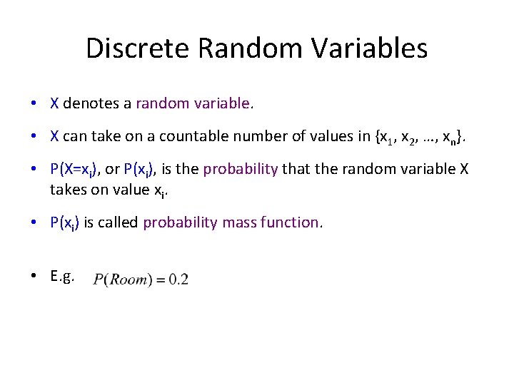
Discrete Random Variables • X denotes a random variable. • X can take on a countable number of values in {x 1, x 2, …, xn}. • P(X=xi), or P(xi), is the probability that the random variable X takes on value xi. • P(xi) is called probability mass function. • E. g.
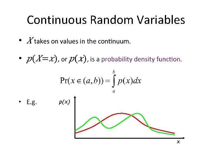
Continuous Random Variables • p(x) x
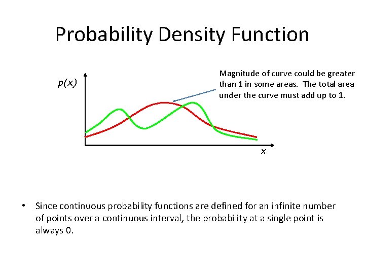
Probability Density Function p(x) Magnitude of curve could be greater than 1 in some areas. The total area under the curve must add up to 1. x • Since continuous probability functions are defined for an infinite number of points over a continuous interval, the probability at a single point is always 0.
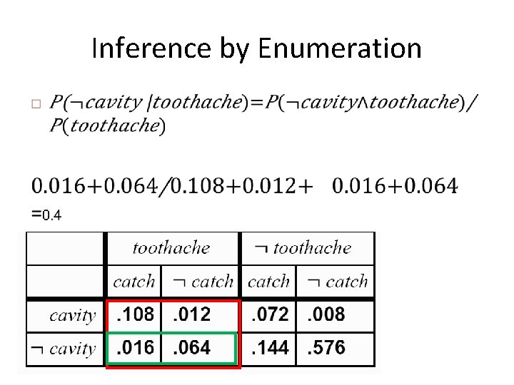
Inference by Enumeration •
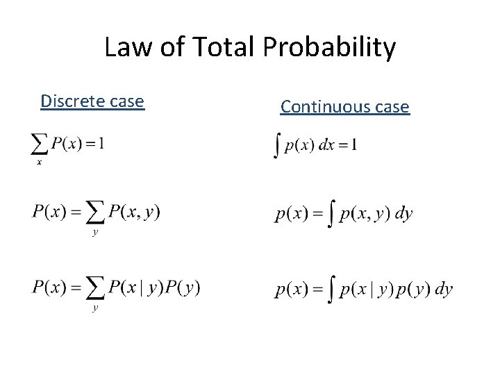
Law of Total Probability Discrete case Continuous case
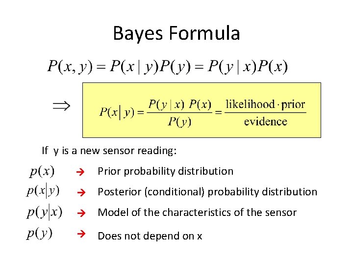
Bayes Formula If y is a new sensor reading: Prior probability distribution Posterior (conditional) probability distribution Model of the characteristics of the sensor Does not depend on x
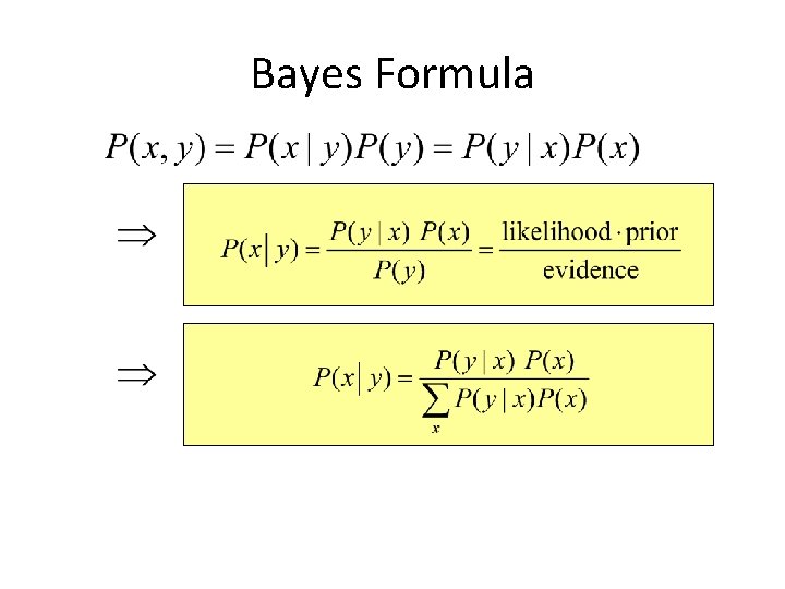
Bayes Formula
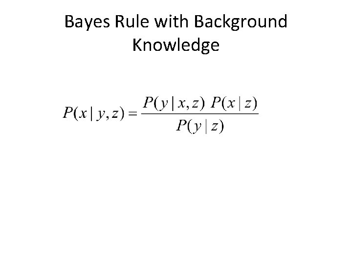
Bayes Rule with Background Knowledge
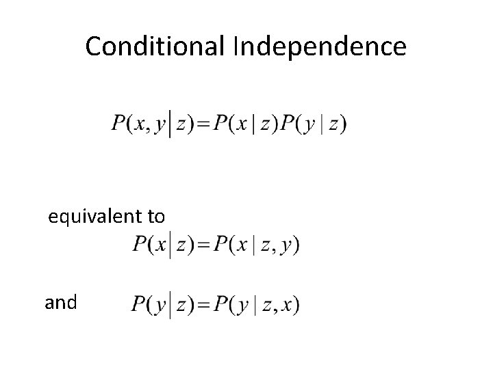
Conditional Independence equivalent to and
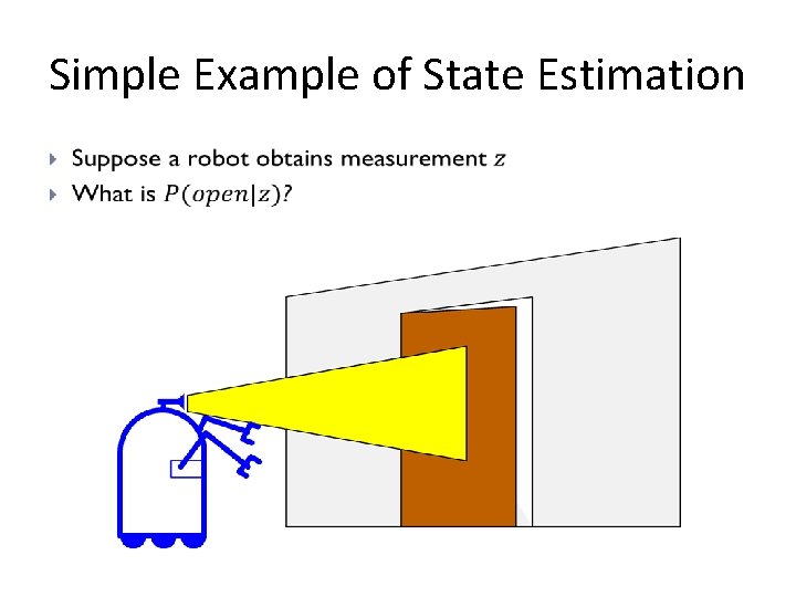
Simple Example of State Estimation •
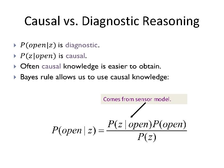
Causal vs. Diagnostic Reasoning • Comes from sensor model.
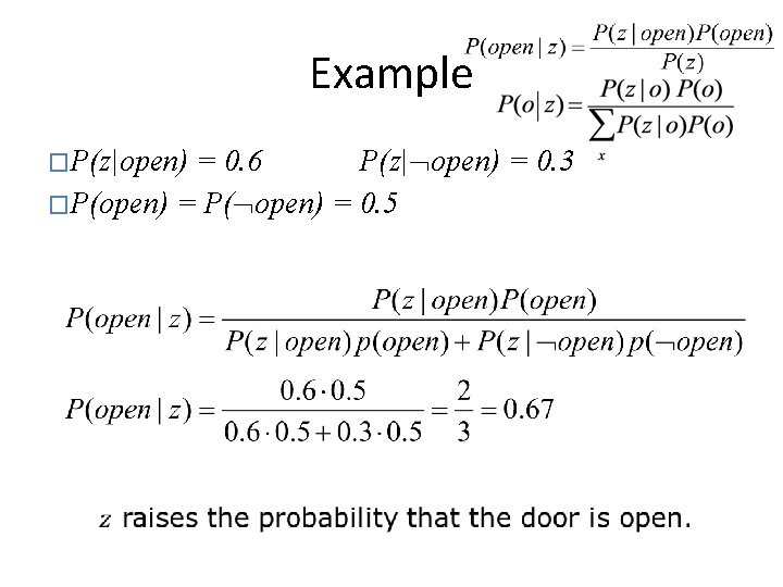
Example �P(z|open) = 0. 6 P(z| open) = 0. 3 �P(open) = P( open) = 0. 5
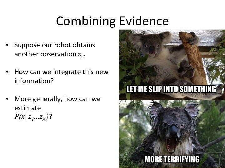
Combining Evidence • Suppose our robot obtains another observation z 2. • How can we integrate this new information? • More generally, how can we estimate P(x| z 1. . . zn )?

Recursive Bayesian Updating Markov assumption: zn is independent of z 1, . . . , zn-1 if we know x.
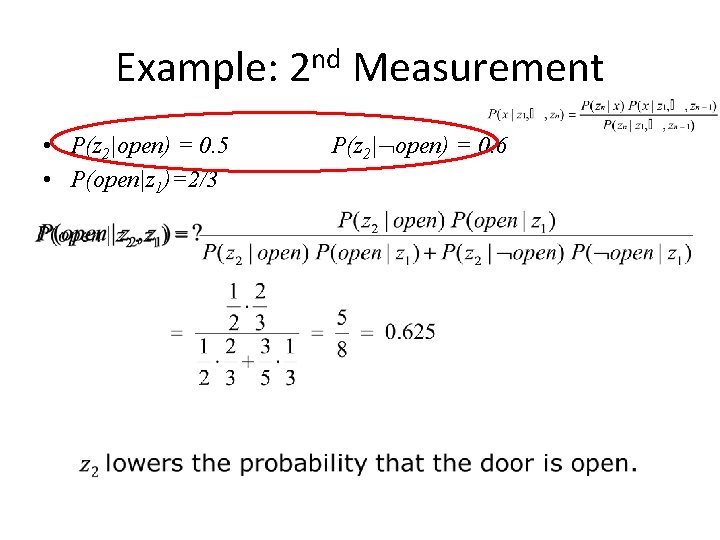
Example: 2 nd Measurement • P(z 2|open) = 0. 5 • P(open|z 1)=2/3 P(z 2| open) = 0. 6
- Slides: 47