Visibility Algorithms Roger Crawfis CIS 781 This set

Visibility Algorithms Roger Crawfis CIS 781 This set of slides reference slides used at Ohio State for instruction by Prof. Machiraju and Prof. Han-Wei Shen.

Visibility Determination • AKA, hidden surface elimination

Hidden Lines

Hidden Lines Removed

Hidden Surfaces Removed

Topics §Backface Culling §Hidden Object Removal: Painters Algorithm §Z-buffer §Spanning Scanline §Warnock §Atherton-Weiler §List Priority, NNA §BSP Tree §Taxonomy
 §Clipping done §division")
Where Are We ? §Canonical view volume (3 D image space) §Clipping done §division by w §z > 0 y y clipped line x 1 1 z image plane near far 0 1 z

Back-face Culling §Problems ? §Conservative algorithm §Real job of visibility never solved

Back-face Culling • If a surface’s normal is pointing in the same general direction as our eye, then this is a back face • The test is quite simple: if N * V > 0 then we reject the surface • If test is in eyespace, then if Nz > 0 reject.

Back-face Culling • Only handles faces oriented away from the viewer: – Closed objects – Near clipping plane does not intersect the objects • Gives complete solution for a single convex polyhedron. • Still need to sort, but we have reduced the number of primitives to sort.
 §Simply overwrite")
Painters Algorithm §Sort objects in depth order §Draw all from Back-to-Front (far-to-near) §Simply overwrite the existing pixels. §Is it so simple?

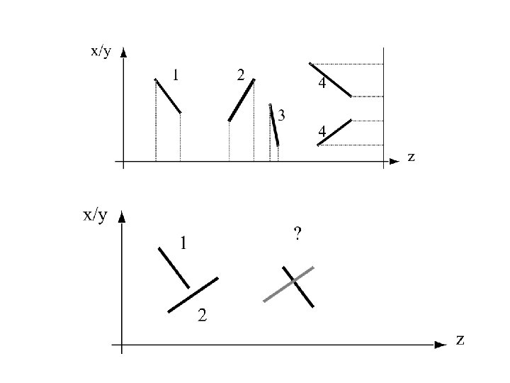
Point sorting vs Polygon Sorting • What does it mean to sort two line segments? – Zmin? – Zmax? – Slope? – Length? z

3 D Cycles §How do we deal with cycles? §How do we deal with intersections? §How do we sort objects that overlap in Z?

Form of the Input Object types: what kind of objects does it handle? § convex vs. non-convex § polygons vs. everything else - smooth curves, noncontinuous surfaces, volumetric data

Form of the output Precision: image/object space? §Object Space §Geometry in, geometry out §Independent of image resolution §Followed by scan conversion §Image Space §Geometry in, image out §Visibility only at pixel centers

Object Space Algorithms § Volume testing – Weiler-Atherton, etc. §input: convex polygons + infinite eye pt §output: visible portions of wireframe edges

Image-space algorithms §Traditional Scan Conversion and Z-buffering § Hierarchical Scan Conversion and Z-buffering §input: any plane-sweepable/plane-boundable objects §preprocessing: none §output: a discrete image of the exact visible set

Conservative Visibility Algorithms §Viewport clipping §Back-face culling §Warnock's screen-space subdivision

Z-buffer §Z-buffer is a 2 D array that stores a depth value for each pixel. §Init. Screen: for i : = 0 to N do for j : = 1 to N do Screen[i][j] : = BACKGROUND_COLOR; Zbuffer[i][j] : = ; §Draw. Zpixel (x, y, z, color) if (z <= Zbuffer[x][y]) then Screen[x][y] : = color; Zbuffer[x][y] : = z;
 in the")
Z-buffer: Scanline I. for each polygon do for each pixel (x, y) in the polygon’s projection do z : = -(D+A*x+B*y)/C; Draw. Zpixel(x, y, z, polygon’s color); II. for each scan-line y do for each “in range” polygon projection do for each pair (x 1, x 2) of X-intersections do for x : = x 1 to x 2 do z : = -(D+A*x+B*y)/C; Draw. Zpixel(x, y, z, polygon’s color); If we know zx, y at (x, y) then: zx+1, y = zx, y - A/C

Incremental Scanline On a scan line Y = j, a constant Thus depth of pixel at (x 1=x+Dx, j) , since Dx = 1,
 § All that was about increment for pixels on each")
Incremental Scanline (contd. ) § All that was about increment for pixels on each scanline. § How about across scanlines for a given pixel ? § Assumption: next scanline is within polygon , since Dy = 1,

Non-Planar Polygons P 3 P 4 ys P 2 za zp zb P 1 Bilinear Interpolation of Depth Values

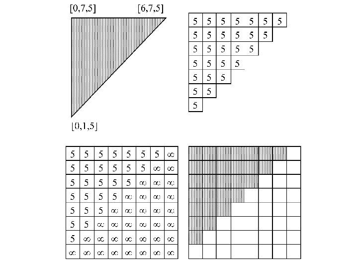
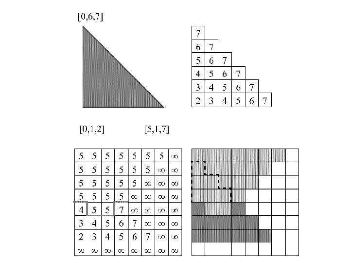
Z-buffer - Example
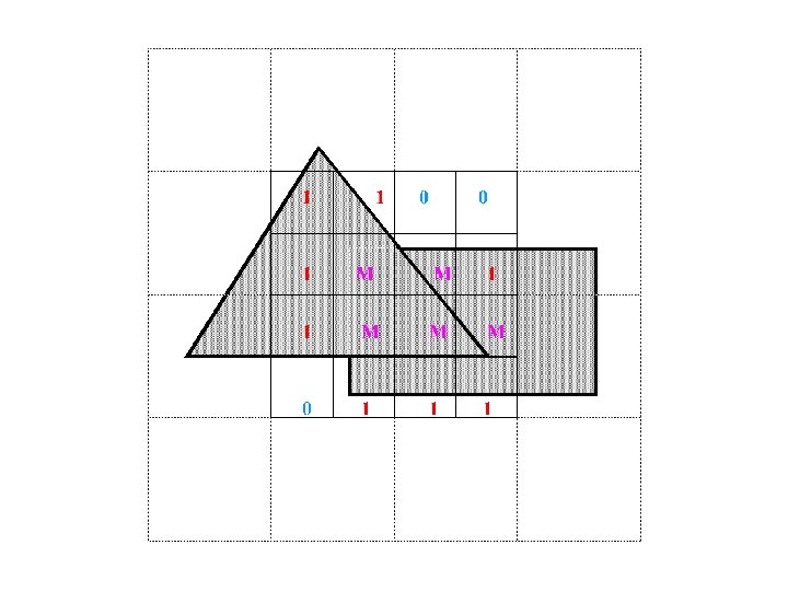
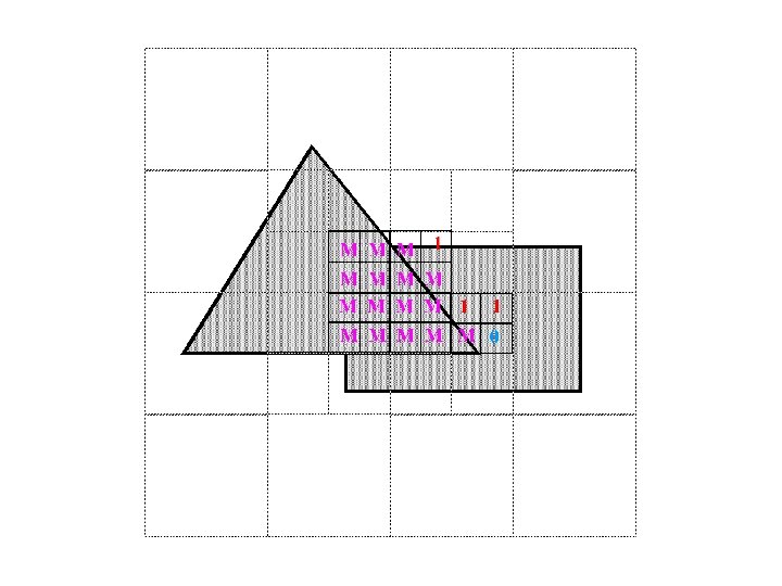
, P 2(10, 25, 10), P")
Non Trivial Example ? Rectangle: P 1(10, 5, 10), P 2(10, 25, 10), P 3(25, 10), P 4(25, 5, 10) Triangle: P 5(15, 15), P 6(25, 5), P 7(30, 10, 5) Frame Buffer: Background 0, Rectangle 1, Triangle 2 Z-buffer: 32 x 4 bit planes

Example

Z-Buffer Advantages § Simple and easy to implement § Amenable to scan-line algorithms § Can easily resolve visibility cycles §Handles intersecting polygons

Z-Buffer Disadvantages § Does not do transparency easily § Aliasing occurs! Since not all depth questions can be resolved § Anti-aliasing solutions non-trivial § Shadows are not easy § Higher order illumination is hard in general

Spanning Scan-Line Can we do better than scan-line Z-buffer ? § Scan-line z-buffer does not exploit §Scan-line coherency across multiple scan-lines §Or span-coherence ! §Depth coherency §How do you deal with this – scan-conversion algorithm and a little more data structure

Spanning Scan Line Algorithm • Use no z-buffer • Each scan line is subdivided into several "spans" • Determine which polygon the current span belongs to • Shade the span using the current polygon’s color • Exploit "span coherence" : • For each span, only one visibility test needs to be done – Assuming no intersecting polygons.

Spanning Scan Line Algorithm • A scan line is subdivided into a sequence of spans • Each span can be "inside" or "outside" polygon areas – "outside“: no pixels need to be drawn (background color) – "inside“: can be inside one or multiple polygons • If a span is inside one polygon, the pixels in the span will be drawn with the color of that polygon • If a span is inside more than one polygon, then we need to compare the z values of those polygons at the scan line edge intersection point to determine the color of the pixel

Spanning Scan Line Algorithm
 • When a scan line")
Determine a span is inside or outside (single polygon) • When a scan line intersects an edge of a polygon – for a 1 st time, the span becomes "inside" of the polygon from that intersection point on – for a 2 nd time, the span becomes "outside“ of the polygon from that point on • Use a "in/out" flag for each polygon to keep track of the current state • Initially, the in/out flag is set to be "outside" (value = 0 for example). Invert the tag for “inside”.

When there are multiple polygons • Each polygon will have its own in/out flag • There can be more than one polygon having the in/out flags to be "in" at a given instance • We want to keep track of how many polygons the scan line is currently in • If there is more than one polygon "in", we need to perform z value comparison to determine the color of the scan line span

Z value comparison • When the scan line intersects an edge, leaving the top-most polygon, we use the color of the remaining polygon if there is now only 1 polygon "in". • If there is still more than one polygon with an "in" flag, we need to perform z comparison, but only when the scan line leaves a non-obscured polygon.

Many Polygons ! § Use a PT entry for each polygon § When polygon is considered, Flag is true § Multiple polygons can have their flags set to true § Use IPL as active In-Polygon List !

Example Think of Scan. Planes to understand !

Spanning Scan-Line: Example Y AET IPL I x 0, ba , bc, x. N BG, BG+S, BG II x 0, ba , bc, 32, 13, x. N BG, BG+S, BG+T, BG III x 0, ba , 32, ca, 13, x. N BG, BG+S+T, BG IV x 0, ba BG, BG+S, BG+T, BG , ac, 12, 13, x. N

Some Facts ! § Scan Line I: Polygon S is in and flag of S=true § Scan. Line II: Both S and T are in and flags are disjointly true § Scan Line III: Both S and T are in simultaneously § Scan Line IV: Same as Scan Line II

Spanning Scan-Line build ET, PT -- all polys+BG poly AET : = IPL : = Nil; for y : = ymin to ymax do e 1 : = first_item ( AET ); IPL : = BG; while (e 1. x <> Max. X) do e 2 : = next_item (AET); poly : = closest poly in IPL at [(e 1. x+e 2. x)/2, y] draw_line(e 1. x, e 2. x, poly-color); update IPL (flags); e 1 : = e 2; end-while; IPL : = NIL; update AET; end-for;

Depth Coherence • Depth relationships may not change between polygons from one scan-line to the next scan-line. • These can be kept track using the (active edge table) AET and the (polgon table) PT. • How about penetrating polygons?

Penetrating Polygons Y AET IPL I x 0, ba , 23, ad, 13, x. N I’ x 0, ba , 23, ec, ad, 13, x. N BG, BG+S+T, BG False edges and new polygons! BG, BG+S, S+T, BG
 Divide and conquer: the relationship of a display area")
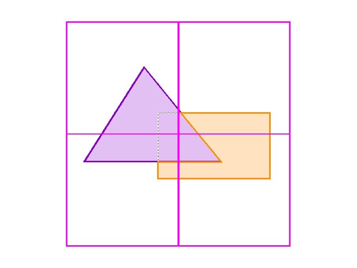
Area Subdivision 1 (Warnock’s Algorithm) Divide and conquer: the relationship of a display area and a polygon after projection is one of the four basic cases:
; else begin if it intersects")
Warnock : One Polygon if it surrounds then draw_rectangle(poly-color); else begin if it intersects then poly : = intersect(poly, rectangle); draw_rectangle(BACKGROUND); draw_poly(poly); end else; What about contained and disjoint ?

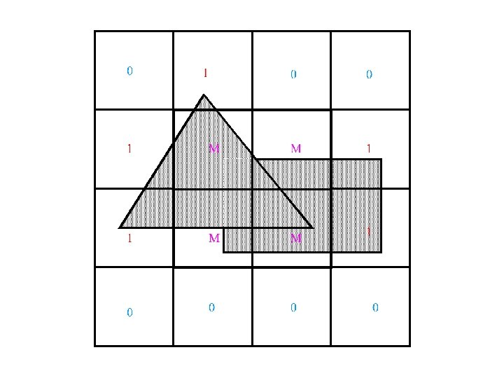
Warnock’s Algorithm • Starting with the entire display, we check the following four cases. If none hold, we subdivide the area and repeat, otherwise, we stop and perform the action associated with the case 1. All polygons are disjoint wrt the area -> draw the background color 2. Only 1 intersecting or contained polygon -> draw background, and then draw the contained portion of the polygon 3. There is a single surrounding polygon -> draw the entire area in the polygon’s color 4. There are more than one intersecting, contained, or surrounding polygons, but there is a front surrounding polygon -> draw the entire area in the polygon’s color • The recursion stops at the pixel level

At A Single Pixel Level • When the recursion stops and none of the four cases hold, we need to perform a depth sort and draw the polygon with the closest Z value • The algorithm is done at the object space level, except scan conversion and clipping are done at the image space level
 new-poly : = clip(rectangle, poly); if new-poly")
Warnock : Zero/One Polygons warnock 01(rectangle, poly) new-poly : = clip(rectangle, poly); if new-poly = NULL then draw_rectangle(BACKGROUND); else draw_rectangle(BACKGROUND); draw_poly(new-poly); return;
 new-list : = clip(rectangle, poly-list); if length(new-list) = 0 then draw_rectangle(BACKGROUND); return;")
Warnock(rectangle, poly-list) new-list : = clip(rectangle, poly-list); if length(new-list) = 0 then draw_rectangle(BACKGROUND); return; if length(new-list) = 1 then draw_rectangle(BACKGROUND); draw_poly(poly); return; if rectangle size = pixel size then poly : = closest polygon at rectangle center draw_rectangle(poly color); return; warnock(top-left quadrant, new-list); warnock(top-right quadrant, new-list); warnock(bottom-left quadrant, new-list); warnock(bottom-right quadrant, new-list);


Area Subdivision 2 Weiler -Atherton Algorithm § Object space § Like Warnock § Output – polygons of arbitrary accuracy

Weiler-Atherton Clipping • General polygon clipping algorithm • Allows one to clip a concave polygon against another concave polygon.

Weiler-Atherton Clipping • First, find all of the intersection points between edges of the two polygons. D B a 6 C c 1 A b 2 4 5 d T S 3 e E S: A, B, C, D, E T: a, b, c, d, e

Weiler-Atherton Clipping • Now, rebuild the polygon’s such that they include the intersection points in their clockwise ordering. D B a 6 C c 1 A b 2 4 5 d T S 3 e E S: A, 1, 4, B, 2, 6, C, D, 5, 3, E T: a, 4, 2, b, 6, c, 5, d, e, 3, 1

Weiler-Atherton Clipping • Find an intersecting vertex of the polygon to be clipped that starts outside and goes inside the clipping region. D • Traverse the polygon until another intersection B point is b 2 4 S: A, 1, 4, B, 2, 6, C, D, 5, 3, E a 6 C found. 5 T: a, 4, 2, b, 6, c, 5, d, e, 3, 1 c d 1 A Clip: 6, c, 5, … T S 3 e E

Weiler-Atherton Clipping • Switch from walking around the polygon 1, to walking around polygon 2, when an intersection is detected. • Stop when we reached the initial point. B a 6 C c 1 A b 2 4 5 d Clip: 6, c, 5, 3, 1, 4, 2, 6 T S 3 e E S: A, 1, 4, B, 2, 6, C, D, 5, 3, E T: a, 4, 2, b, 6, c, 5, d, e, 3, 1

Weiler -Atherton Algorithm • • Subdivide along polygon boundaries (unlike Warnock’s rectangular boundaries in image space); Algorithm: 1. Sort the polygons based on their minimum z distance 2. Choose the first polygon P in the sorted list 3. Clip all polygons left against P, create two lists: – Inside list: polygon fragments inside P (including P) – Outside list: polygon fragments outside P 4. All polygon fragments on the inside list that are behind P are discarded. If there are polygons on the inside list that are in front of P, go back to step 3), use the ’offending’ polygons as P 5. Display P and go back to step (2)
 sort_by_min. Z(polys); while (polys <> NULL)")
Weiler -Atherton Algorithm WA_display(polys : List. Of. Polygons) sort_by_min. Z(polys); while (polys <> NULL) do WA_subdiv(polys->first, polys) end; WA_subdiv(first: Polygon; polys: List. Of. Polygons) in. P, out. P : List. Of. Polygons : = NULL; for each P in polys do Clip(P, first->ancestor, in. P, out. P); for each P in in. P do if P is behind (min z)first then discard P; for each P in in. P do if P is not part of first then for each P in in. P do display_a_poly(P); polys : = out. P; end; WA_subdiv(P, in. P);


List Priority Algorithms • Find a valid order for rendering. • Only consider cases where the sort matters.

List Priority Algorithms §If objects do not overlap in X or in Y there is no need for hidden object removal process. §If they do not overlap in the Z dimension they can be sorted by Z and rendered in back (highest priority)-tofront (lowest priority) order (Painter’s Algorithm). §It is easy then to implement transparency. §How do we sort ? – different algorithms differ
![Newell, Sancha Algorithm 1. Sort by [minz. . maxz] of each polygon 2. For](http://slidetodoc.com/presentation_image_h2/1bece40be0f336b9b8de30f71b9ea115/image-69.jpg "Newell, Sancha Algorithm 1. Sort by [minz. . maxz] of each polygon 2. For")
Newell, Sancha Algorithm 1. Sort by [minz. . maxz] of each polygon 2. For each group of unsorted polygons G resolve_ambiguities(G); 3. Render polygons in a back-to-front order. resolve_ambiguities is basically a sorting algorithm that relies on the procedure rearrange(P, Q): resolve_ambiguities(G) not-yet-done : = TRUE; while (not-yet-done) do not-yet-done : = FALSE; for each pair of polygons P, Q in G do --- bubble sort L : = rearrange(P, Q, not-yet-done); insert L into G instead of P, Q
 if (P and Q do not have overlapping")
Newell, Sancha Algorithm rearrange(P, Q, flag) if (P and Q do not have overlapping x-extents, return P, Q if (P and Q do not have overlapping y-extents, return P, Q if all Q is on the opposite side of P from the eye return P, Q if all P is on the same side of Q from the eye return P, Q if not overlap-projection(P, Q) return P, Q flag : = TRUE; // more work is needed if all Q is on the same side of P from the eye return Q, P if all P is on the opposite side of Q from the eye return Q, P split(P, Q, p 1, p 2); return (p 1, p 2, Q); -- split P by Q

Newell-Sancha Sorting • Q is on the opposite side of P. • Means, all of Q’s vertices are behind the half-plane defined by P. P P Q Q True False

Newell-Sancha Sorting • P is on the same side of Q. • Means, all of P’s vertices are in front of the half-plane defined by Q. P P Q Q False True
 Image Space")
Taxonomy A characterization of 10 Hidden Surface Algorithm: Sutherland, Sproull, Schumaker (1974) Image Space Object space List priority edge volume Area Point A’priori Dynamic Apel, Weiler-Atherton Roberts Newell Warnock Span-line Algorithms

Spatial Subdivision • • • Uniform grid Octrees K-d Trees BSP-trees Non-overlapping polyhedra – Axis-Aligned Bounding Boxes (AABB’s) – Oriented Bounding Boxes (OBB’s) – Useful for non-static scenes

Back-to-front Traversals • For the first four, you can develop either a front-to-back or back-to-front traversal order explicitly. • Thereby, solving the visibility sort efficiently. • For the polyhedra, use a Newell-Newell. Sancha sort.

Sorting for Uniform Grid • Parallel Projection – Can always proceed along the x-axis, then yaxis then z-axis or any combination. – Simply need to decide whether to go forward or backward on each axis. • Look at the z-value of the transformed x-axis, … • Positive, go forward for back-to-front sort. – Better ordering would choose the axis most parallel to the viewing direction to traverse last.

Sorting for Uniform Grid • Perspective projection – May need to proceed forward for part of the grid and backwards for the other.

K-d Trees • Alternate splits in each direction Split X axis Split Y axis X

K-d Trees • Extend to any dimension d • In 3 D, the splits are done with axis-aligned planes. – Test is simple, is x-value (for nodes splitting the x-axis) greater than the node value?

K-d Trees • A subset of BSP-trees. • Sorting is the same. • More efficient storage representation.

Binary Space-Partitioning Tree §Given a polygon p §Two lists of polygons: §those that are behind(p) : B §those that are in-front(p) : F § If eye is in-front(p), right display order is B, p, F §Otherwise it is F, p, B
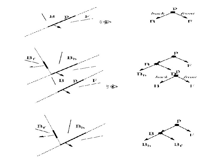

Display a BSP Tree struct bspnode { p: Polygon; back, front : *bspnode; } BSPTree; BSP_display ( bspt ) BSPTree *bspt; { if (!bspt) return; if (Eye. Infront. Poly( bspt->p )) { BSP_display(bspt->back); Poly_display(bspt->p); BSP_display(bspt->front); } else { BSP_display(bspt->front); Poly_display(bspt->p); BSP_display(bspt->back); } }
 then return NULL; rootp :")
Generating a BSP Tree if (polys is empty ) then return NULL; rootp : = first polygon in polys; for each polygon p in the rest of polys do if p is infront of rootp then add p to the front list else if p is in the back of rootp then add p to the back list else split p into a back poly pb and front poly pf add pf to the front list add pb to the back list end_for; bspt->back : = BSP_gentree(back list); bspt->front : = BSP_gentree(front list); bspt->p = rootp; return bspt;

- Slides: 85