Viscous flow in ducts Circular and noncircular ducts

Viscous flow in ducts

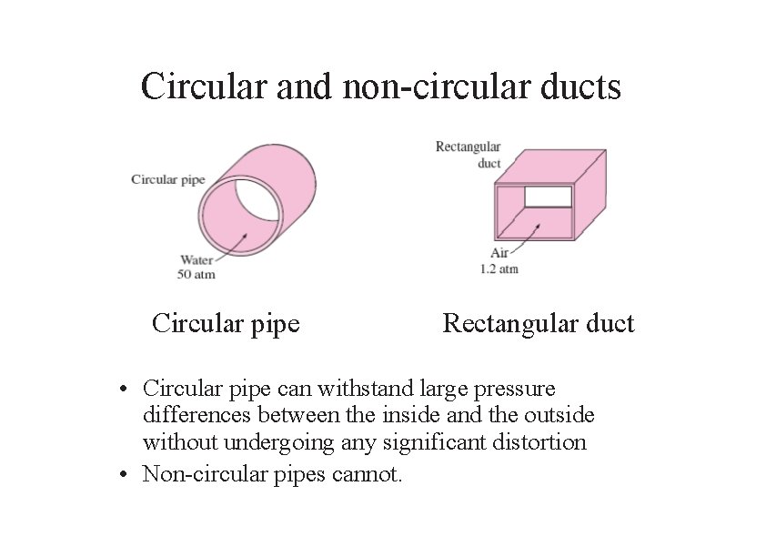
Circular and non-circular ducts Circular pipe Rectangular duct • Circular pipe can withstand large pressure differences between the inside and the outside without undergoing any significant distortion • Non-circular pipes cannot.

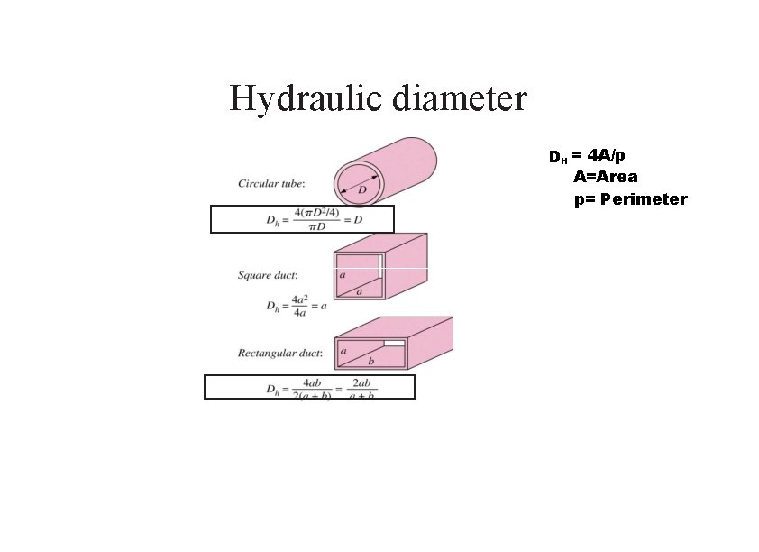
Hydraulic diameter DH = 4 A/p A=Area p= Perimeter

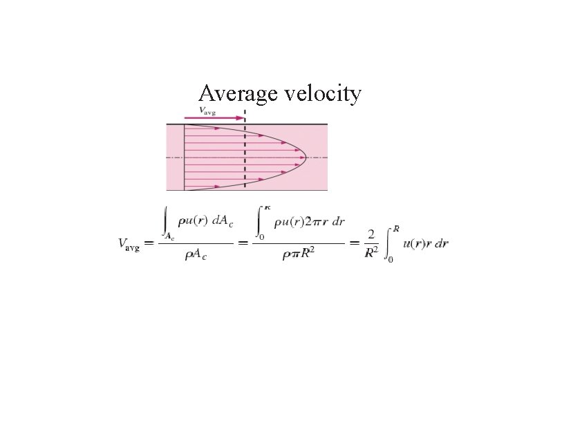
Average velocity

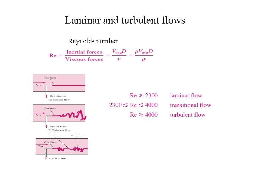
Laminar and turbulent flows Reynolds number

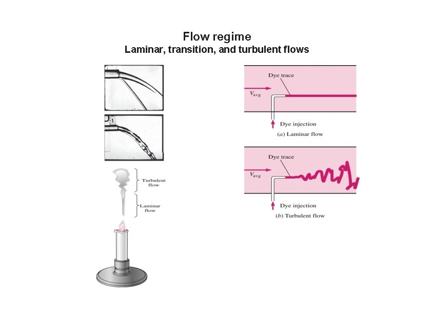
Flow regime Laminar, transition, and turbulent flows

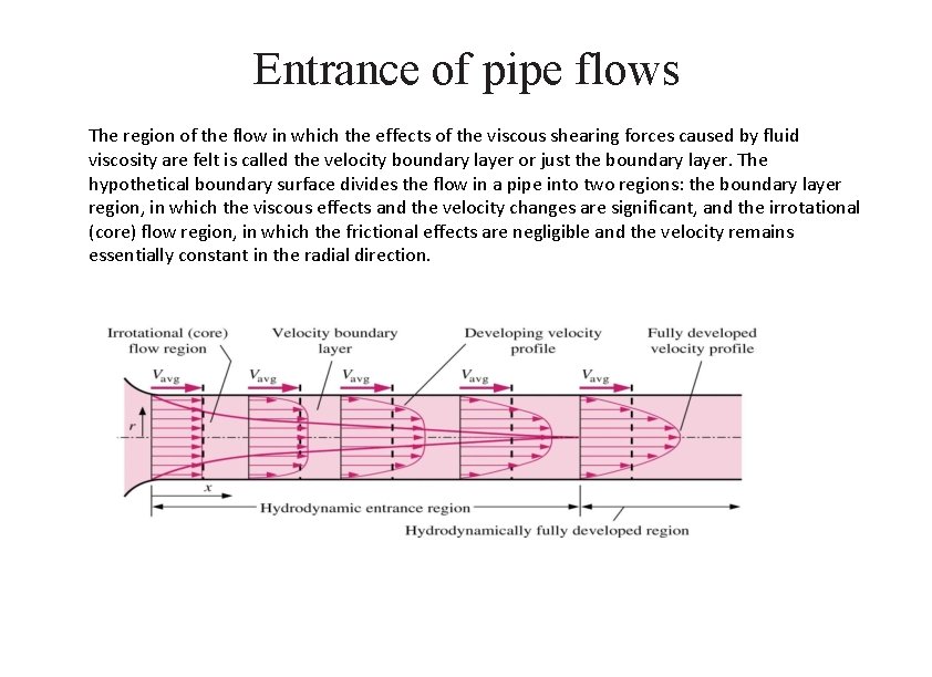
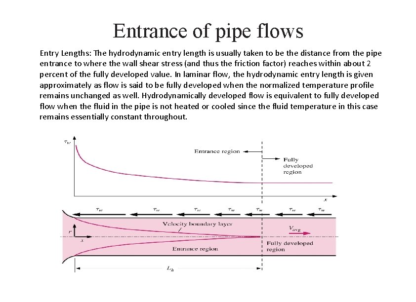
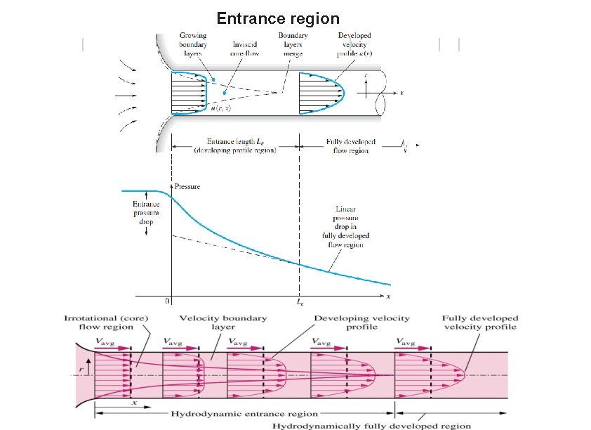
Entrance of pipe flows The region of the flow in which the effects of the viscous shearing forces caused by fluid viscosity are felt is called the velocity boundary layer or just the boundary layer. The hypothetical boundary surface divides the flow in a pipe into two regions: the boundary layer region, in which the viscous effects and the velocity changes are significant, and the irrotational (core) flow region, in which the frictional effects are negligible and the velocity remains essentially constant in the radial direction.

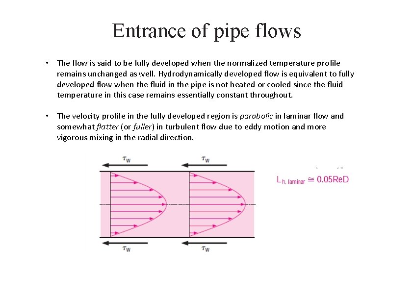
Entrance of pipe flows • The flow is said to be fully developed when the normalized temperature profile remains unchanged as well. Hydrodynamically developed flow is equivalent to fully developed flow when the fluid in the pipe is not heated or cooled since the fluid temperature in this case remains essentially constant throughout. • The velocity profile in the fully developed region is parabolic in laminar flow and somewhat flatter (or fuller) in turbulent flow due to eddy motion and more vigorous mixing in the radial direction.

Entrance of pipe flows Entry Lengths: The hydrodynamic entry length is usually taken to be the distance from the pipe entrance to where the wall shear stress (and thus the friction factor) reaches within about 2 percent of the fully developed value. In laminar flow, the hydrodynamic entry length is given approximately as flow is said to be fully developed when the normalized temperature profile remains unchanged as well. Hydrodynamically developed flow is equivalent to fully developed flow when the fluid in the pipe is not heated or cooled since the fluid temperature in this case remains essentially constant throughout.

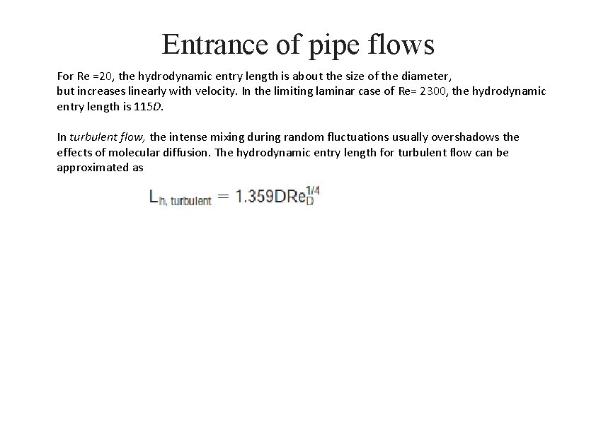
Entrance of pipe flows For Re =20, the hydrodynamic entry length is about the size of the diameter, but increases linearly with velocity. In the limiting laminar case of Re= 2300, the hydrodynamic entry length is 115 D. In turbulent flow, the intense mixing during random fluctuations usually overshadows the effects of molecular diffusion. The hydrodynamic entry length for turbulent flow can be approximated as

Entrance region

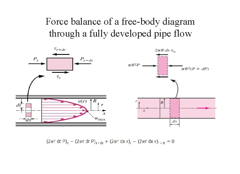
Force balance of a free-body diagram through a fully developed pipe flow

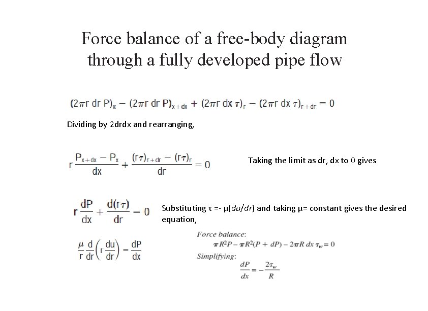
Force balance of a free-body diagram through a fully developed pipe flow Dividing by 2 drdx and rearranging, Taking the limit as dr, dx to 0 gives Substituting τ =- µ(du/dr) and taking µ= constant gives the desired equation,

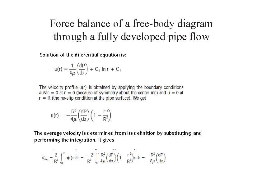
Force balance of a free-body diagram through a fully developed pipe flow Solution of the diferential equation is: The average velocity is determined from its definition by substituting and performing the integration. It gives

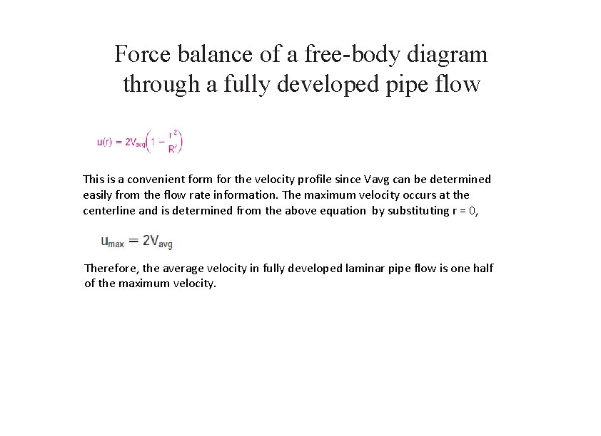
Force balance of a free-body diagram through a fully developed pipe flow This is a convenient form for the velocity profile since Vavg can be determined easily from the flow rate information. The maximum velocity occurs at the centerline and is determined from the above equation by substituting r = 0, Therefore, the average velocity in fully developed laminar pipe flow is one half of the maximum velocity.

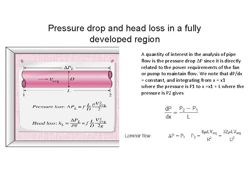
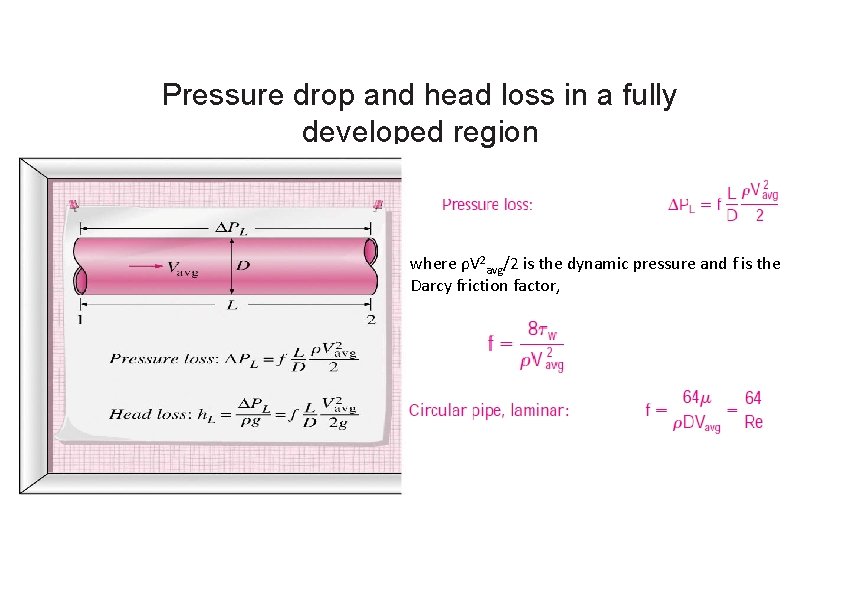
Pressure drop and head loss in a fully developed region A quantity of interest in the analysis of pipe flow is the pressure drop ΔP since it is directly related to the power requirements of the fan or pump to maintain flow. We note that d. P/dx = constant, and integrating from x = x 1 where the pressure is P 1 to x =x 1 + L where the pressure is P 2 gives

Pressure drop and head loss in a fully developed region where ρV 2 avg/2 is the dynamic pressure and f is the Darcy friction factor,

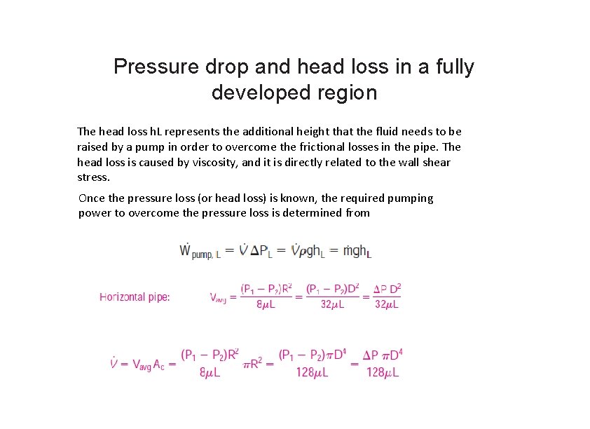
Pressure drop and head loss in a fully developed region The head loss h. L represents the additional height that the fluid needs to be raised by a pump in order to overcome the frictional losses in the pipe. The head loss is caused by viscosity, and it is directly related to the wall shear stress. Once the pressure loss (or head loss) is known, the required pumping power to overcome the pressure loss is determined from

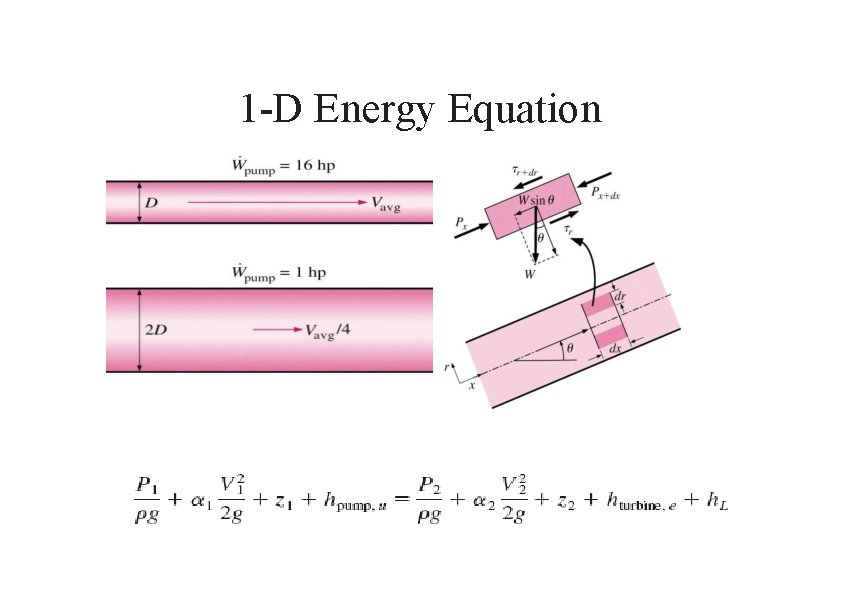
1 -D Energy Equation

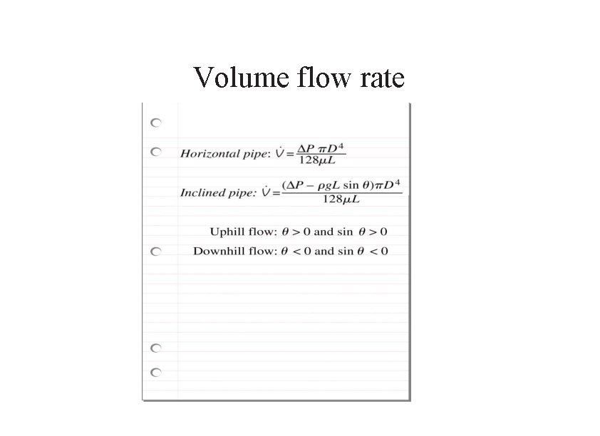
Volume flow rate

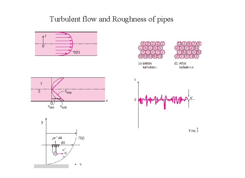
Turbulent flow and Roughness of pipes

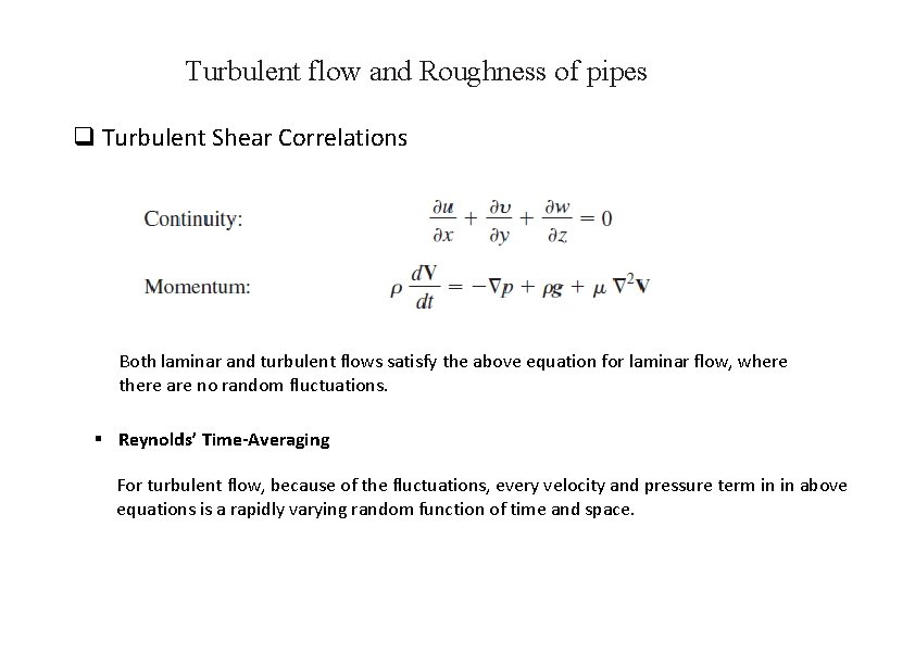
Turbulent flow and Roughness of pipes q Turbulent Shear Correlations Both laminar and turbulent flows satisfy the above equation for laminar flow, where there are no random fluctuations. § Reynolds’ Time-Averaging For turbulent flow, because of the fluctuations, every velocity and pressure term in in above equations is a rapidly varying random function of time and space.

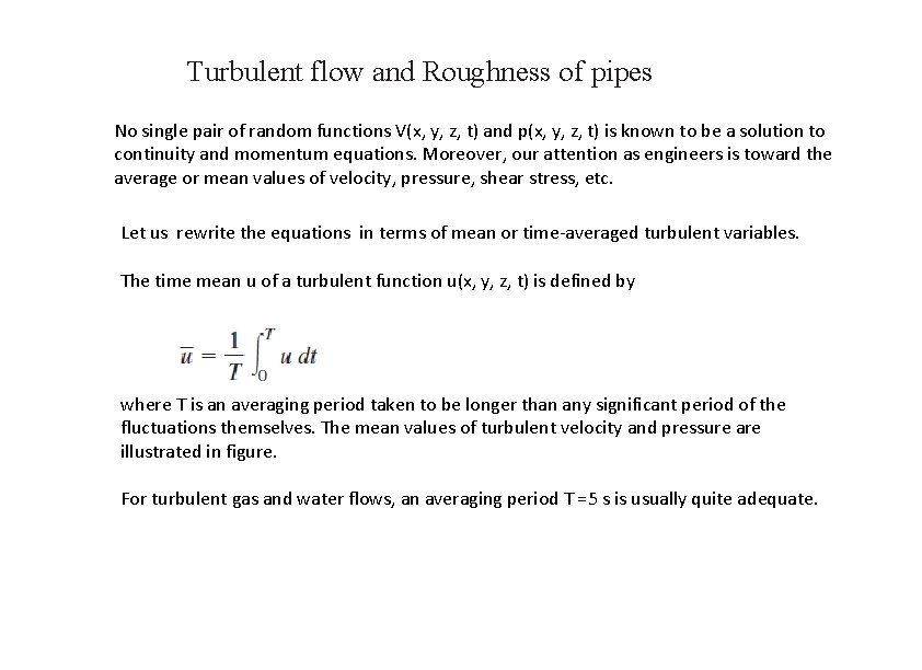
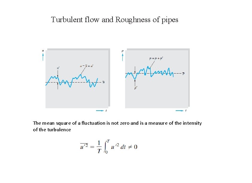
Turbulent flow and Roughness of pipes No single pair of random functions V(x, y, z, t) and p(x, y, z, t) is known to be a solution to continuity and momentum equations. Moreover, our attention as engineers is toward the average or mean values of velocity, pressure, shear stress, etc. Let us rewrite the equations in terms of mean or time-averaged turbulent variables. The time mean u of a turbulent function u(x, y, z, t) is defined by where T is an averaging period taken to be longer than any significant period of the fluctuations themselves. The mean values of turbulent velocity and pressure are illustrated in figure. For turbulent gas and water flows, an averaging period T =5 s is usually quite adequate.

Turbulent flow and Roughness of pipes The mean square of a fluctuation is not zero and is a measure of the intensity of the turbulence

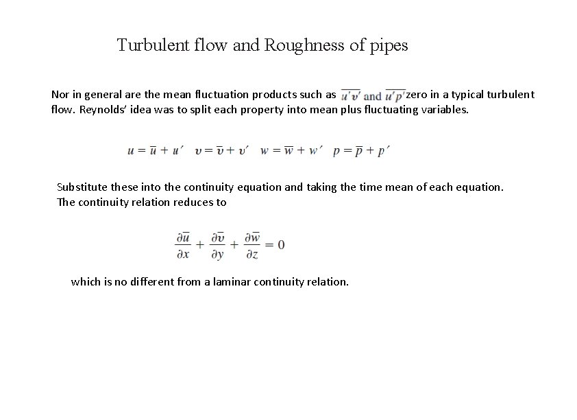
Turbulent flow and Roughness of pipes Nor in general are the mean fluctuation products such as zero in a typical turbulent flow. Reynolds’ idea was to split each property into mean plus fluctuating variables. Substitute these into the continuity equation and taking the time mean of each equation. The continuity relation reduces to which is no different from a laminar continuity relation.

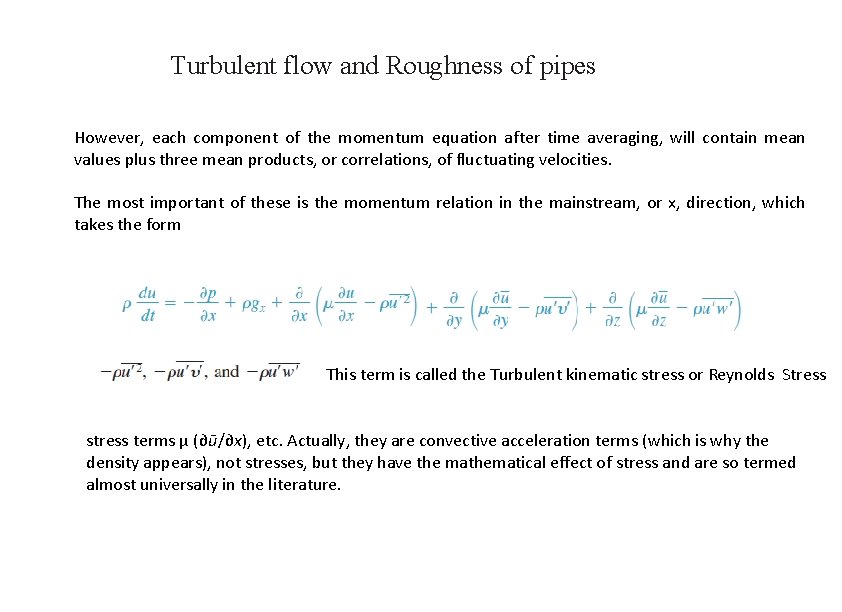
Turbulent flow and Roughness of pipes However, each component of the momentum equation after time averaging, will contain mean values plus three mean products, or correlations, of fluctuating velocities. The most important of these is the momentum relation in the mainstream, or x, direction, which takes the form This term is called the Turbulent kinematic stress or Reynolds Stress stress terms μ (∂ū/∂x), etc. Actually, they are convective acceleration terms (which is why the density appears), not stresses, but they have the mathematical effect of stress and are so termed almost universally in the literature.

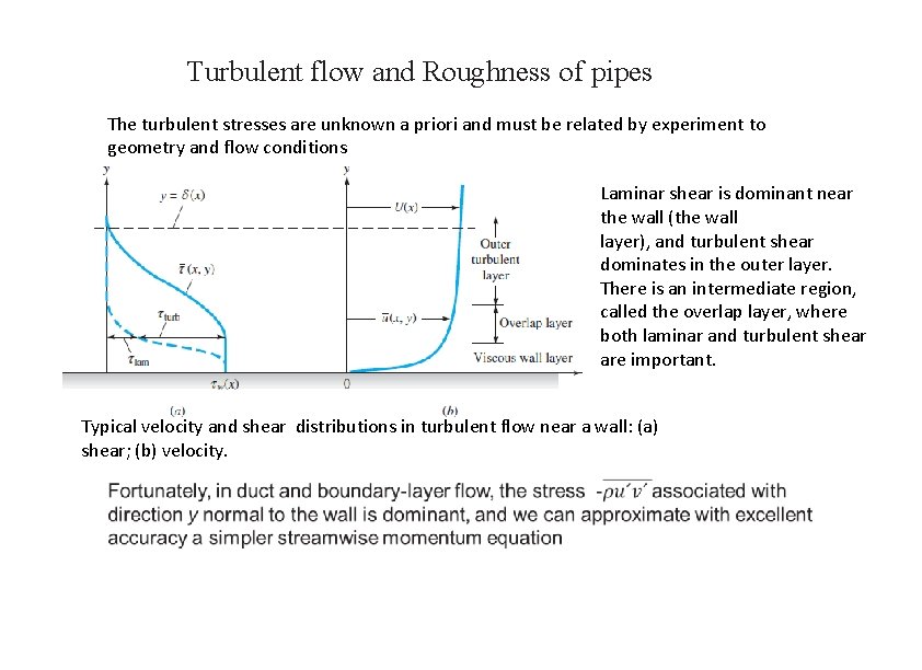
Turbulent flow and Roughness of pipes The turbulent stresses are unknown a priori and must be related by experiment to geometry and flow conditions Laminar shear is dominant near the wall (the wall layer), and turbulent shear dominates in the outer layer. There is an intermediate region, called the overlap layer, where both laminar and turbulent shear are important. Typical velocity and shear distributions in turbulent flow near a wall: (a) shear; (b) velocity.

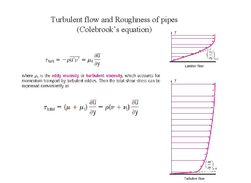
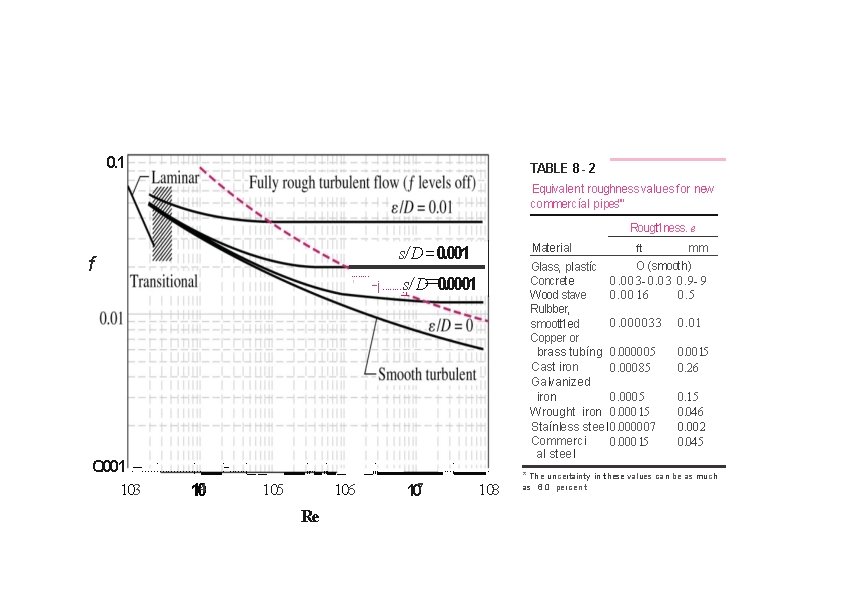
Turbulent flow and Roughness of pipes (Colebrook’s equation)

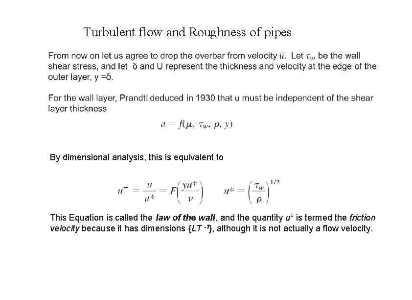
Turbulent flow and Roughness of pipes The Logarithmic-Overlap Law We have seen in above figure that there are three regions in turbulent flow near a wall: 1. Wall layer: Viscous shear dominates. 2. Outer layer: Turbulent shear dominates. 3. Overlap layer: Both types of shear are important.

Turbulent flow and Roughness of pipes By dimensional analysis, this is equivalent to This Equation is called the law of the wall, and the quantity u* is termed the friction velocity because it has dimensions {LT -1}, although it is not actually a flow velocity.

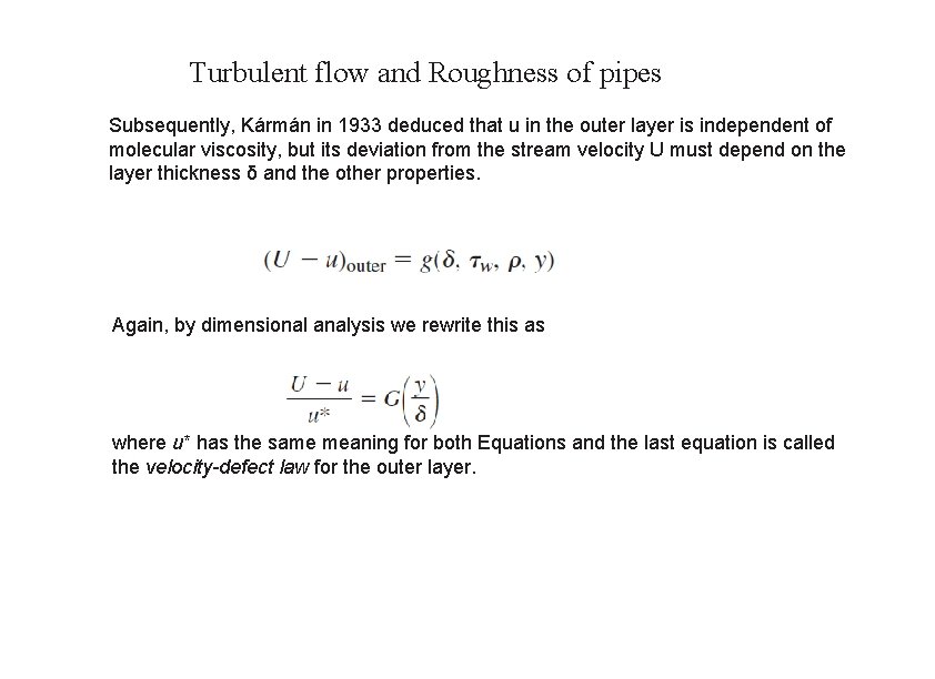
Turbulent flow and Roughness of pipes Subsequently, Kármán in 1933 deduced that u in the outer layer is independent of molecular viscosity, but its deviation from the stream velocity U must depend on the layer thickness δ and the other properties. Again, by dimensional analysis we rewrite this as where u* has the same meaning for both Equations and the last equation is called the velocity-defect law for the outer layer.

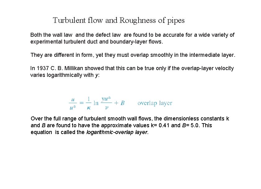
Turbulent flow and Roughness of pipes Both the wall law and the defect law are found to be accurate for a wide variety of experimental turbulent duct and boundary-layer flows. They are different in form, yet they must overlap smoothly in the intermediate layer. In 1937 C. B. Millikan showed that this can be true only if the overlap-layer velocity varies logarithmically with y: Over the full range of turbulent smooth wall flows, the dimensionless constants k and B are found to have the approximate values k= 0. 41 and B= 5. 0. This equation is called the logarithmic-overlap layer.

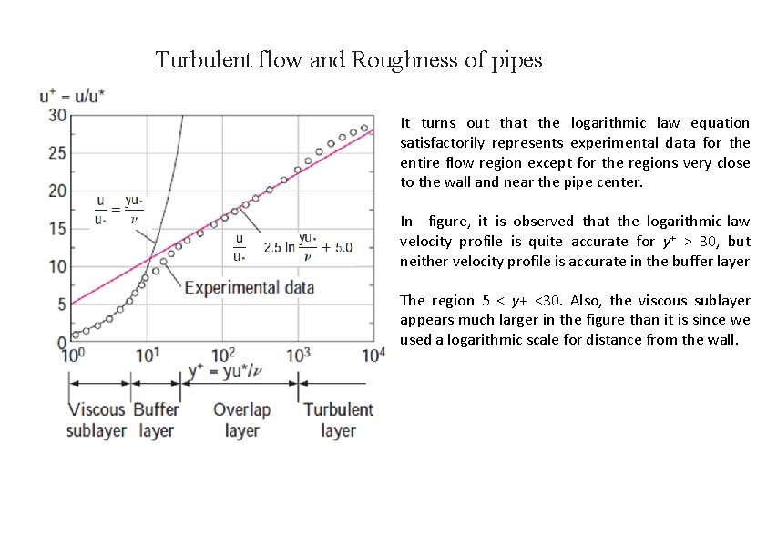
Turbulent flow and Roughness of pipes It turns out that the logarithmic law equation satisfactorily represents experimental data for the entire flow region except for the regions very close to the wall and near the pipe center. In figure, it is observed that the logarithmic-law velocity profile is quite accurate for y+ > 30, but neither velocity profile is accurate in the buffer layer The region 5 < y+ <30. Also, the viscous sublayer appears much larger in the figure than it is since we used a logarithmic scale for distance from the wall.

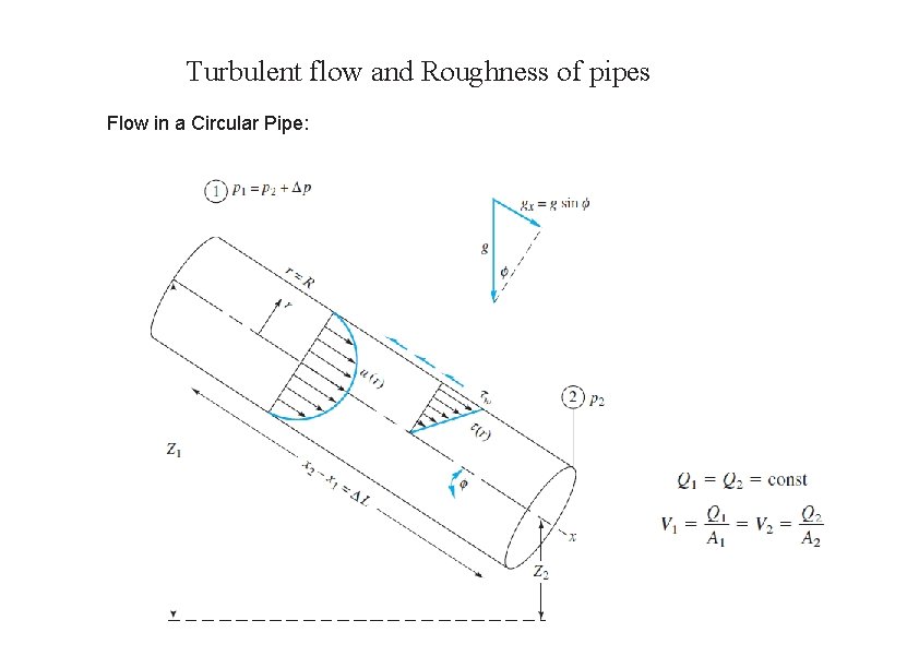
Turbulent flow and Roughness of pipes Flow in a Circular Pipe:

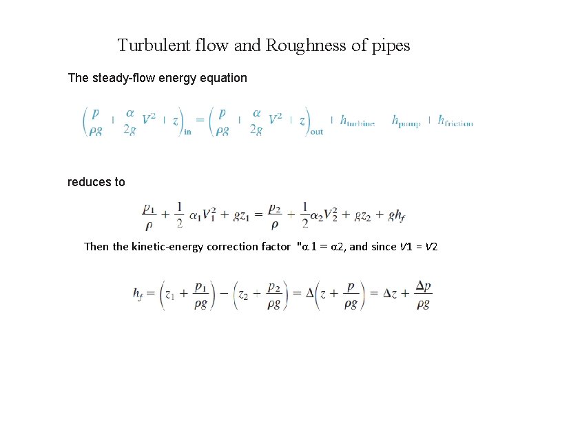
Turbulent flow and Roughness of pipes The steady-flow energy equation reduces to Then the kinetic-energy correction factor "α 1 = α 2, and since V 1 = V 2

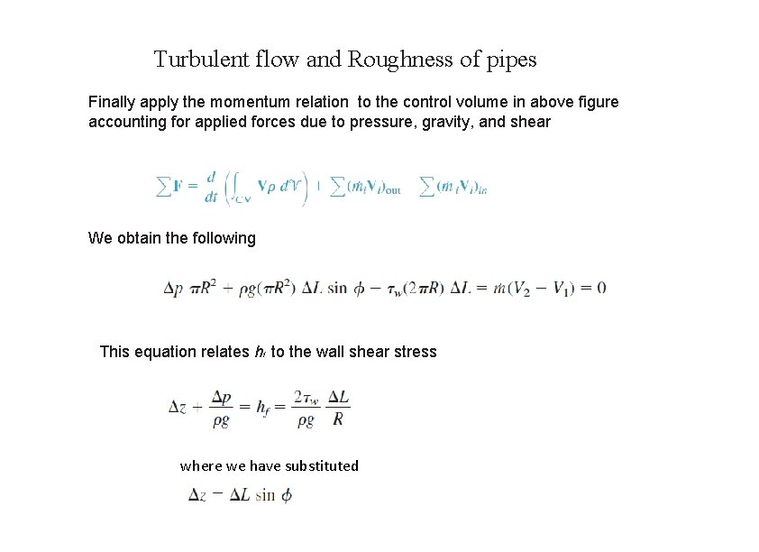
Turbulent flow and Roughness of pipes Finally apply the momentum relation to the control volume in above figure accounting for applied forces due to pressure, gravity, and shear We obtain the following This equation relates hf to the wall shear stress where we have substituted

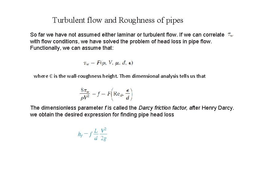
Turbulent flow and Roughness of pipes So far we have not assumed either laminar or turbulent flow. If we can correlate with flow conditions, we have solved the problem of head loss in pipe flow. Functionally, we can assume that: where Є is the wall-roughness height. Then dimensional analysis tells us that The dimensionless parameter f is called the Darcy friction factor, after Henry Darcy. we obtain the desired expression for finding pipe head loss

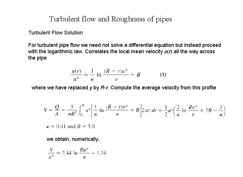
Turbulent flow and Roughness of pipes Turbulent Flow Solution For turbulent pipe flow we need not solve a differential equation but instead proceed with the logarithmic law. Correlates the local mean velocity u(r) all the way across the pipe (1) where we have replaced y by R-r. Compute the average velocity from this profile we obtain, numerically,

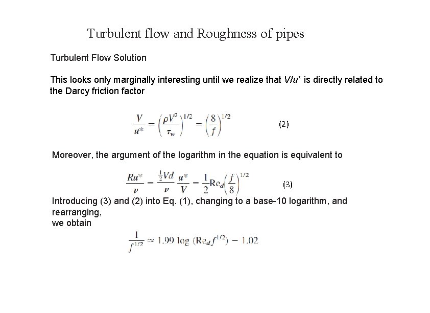
Turbulent flow and Roughness of pipes Turbulent Flow Solution This looks only marginally interesting until we realize that V/u* is directly related to the Darcy friction factor (2) Moreover, the argument of the logarithm in the equation is equivalent to (3) Introducing (3) and (2) into Eq. (1), changing to a base-10 logarithm, and rearranging, we obtain

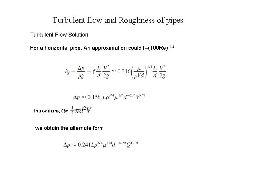
Turbulent flow and Roughness of pipes Turbulent Flow Solution For a horizontal pipe, An approximation could f=(100 Re)-1/4 Introducing Q= we obtain the alternate form

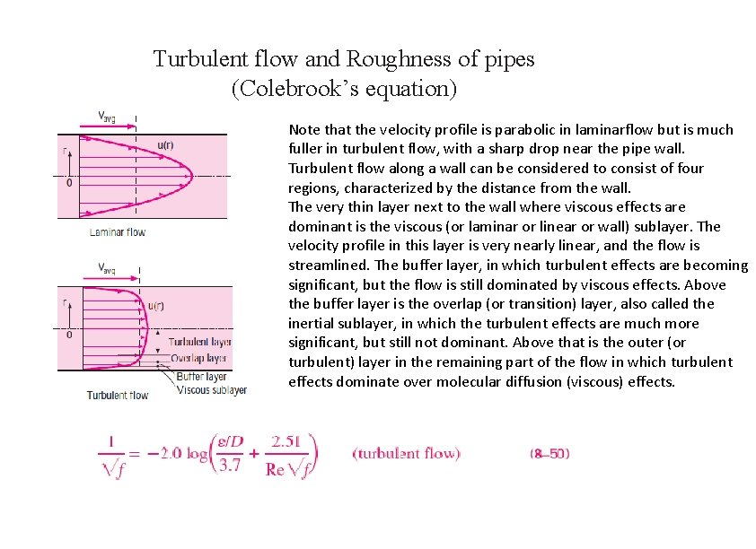
Turbulent flow and Roughness of pipes (Colebrook’s equation) Note that the velocity profile is parabolic in laminarflow but is much fuller in turbulent flow, with a sharp drop near the pipe wall. Turbulent flow along a wall can be considered to consist of four regions, characterized by the distance from the wall. The very thin layer next to the wall where viscous effects are dominant is the viscous (or laminar or linear or wall) sublayer. The velocity profile in this layer is very nearly linear, and the flow is streamlined. The buffer layer, in which turbulent effects are becoming significant, but the flow is still dominated by viscous effects. Above the buffer layer is the overlap (or transition) layer, also called the inertial sublayer, in which the turbulent effects are much more significant, but still not dominant. Above that is the outer (or turbulent) layer in the remaining part of the flow in which turbulent effects dominate over molecular diffusion (viscous) effects.

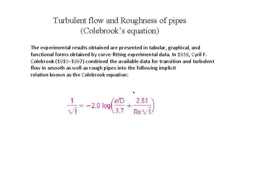
Turbulent flow and Roughness of pipes (Colebrook’s equation) The experimental results obtained are presented in tabular, graphical, and functional forms obtained by curve-fitting experimental data. In 1939, Cyril F. Colebrook (1910– 1997) combined the available data for transition and turbulent flow in smooth as well as rough pipes into the following implicit relation known as the Colebrook equation:

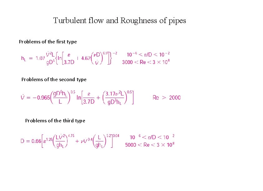
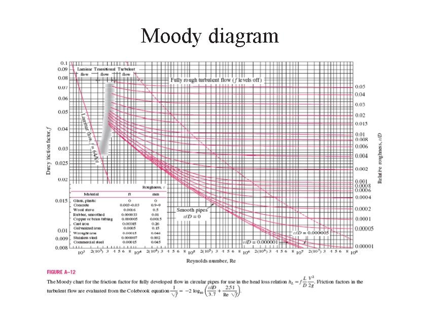
Turbulent flow and Roughness of pipes We usually encounter three types of problems, the fluid and the roughness of the pipe are assumed to be specified in all cases. 1. Determining the pressure drop (or head loss) when the pipe length and diameter are given for a specified flow rate (or velocity). 2. Determining the flow rate when the pipe length and diameter are given for a specified pressure drop (or head loss). 3. Determining the pipe diameter when the pipe length and flow rate are given for a specified pressure drop (or head loss). Problems of the first type are straightforward and can be solved directly by using the Moody chart. Problems of the second type and third type are commonly encountered in engineering design

Turbulent flow and Roughness of pipes Problems of the first type Problems of the second type Problems of the third type

Moody diagram

0. 1 TABLE 8 - 2 Equivalent roughness values for new commercíal pipes"" Rougt 1 ness. e f O. 001. --. . . : . . . ; . . : -. . . ; _ _ 105 103 104 Material s/D = 0. 001. . . . 1 -¡. . . . _. s/ , D=0. 0001 ; , . . . , ; , _ _, ; , 106 Re . . . ; 107 . 108 ft mm O (smooth) Glass, plastíc Concrete 0. 003 - 0. 03 0. 9 - 9 0. 00 16 0. 5 Wood stave Rulbber, 0. 000033 0. 01 smoott 1 ed Copper or brass tubíng 0. 000005 0. 0015 Cast iron 0. 00085 0. 26 Galvanized iron 0. 0005 0. 15 Wrought iron 0. 00015 0. 046 Staínless stee l 0. 000007 0. 002 Commerci 0. 00015 0. 045 al steel * The uncertainty in t hese val ues can be as much as 6 0 percent

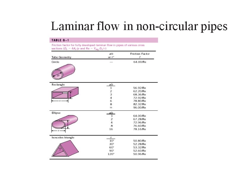
Laminar flow in non-circular pipes

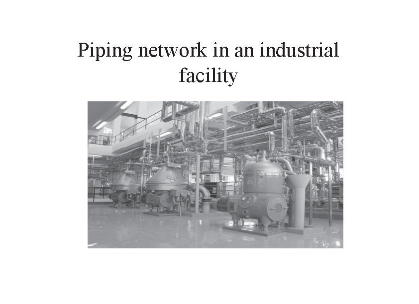
Piping network in an industrial facility

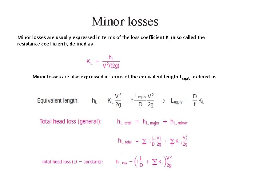
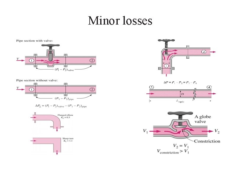
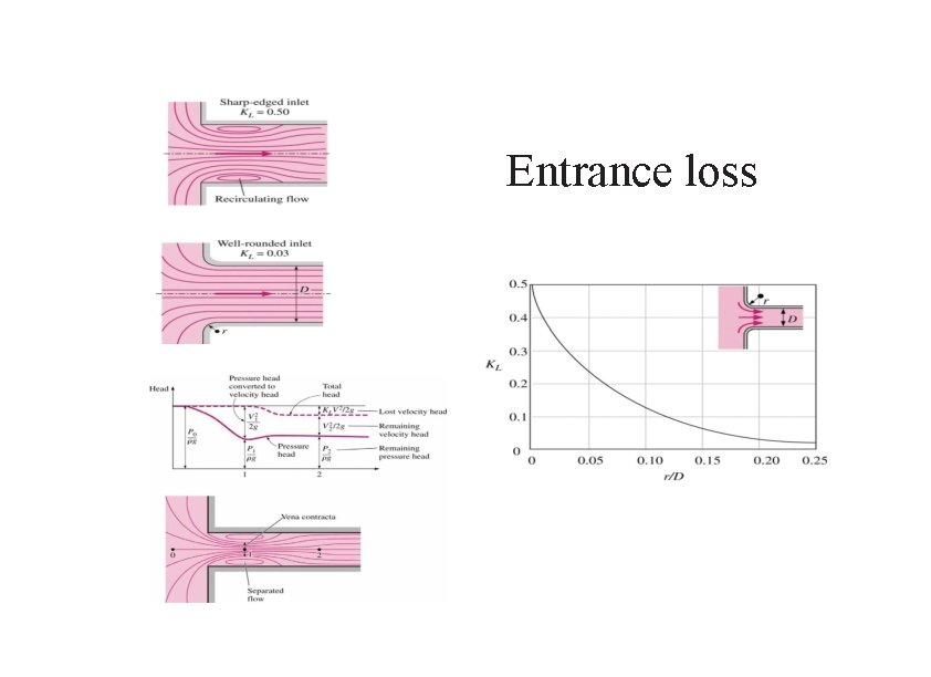
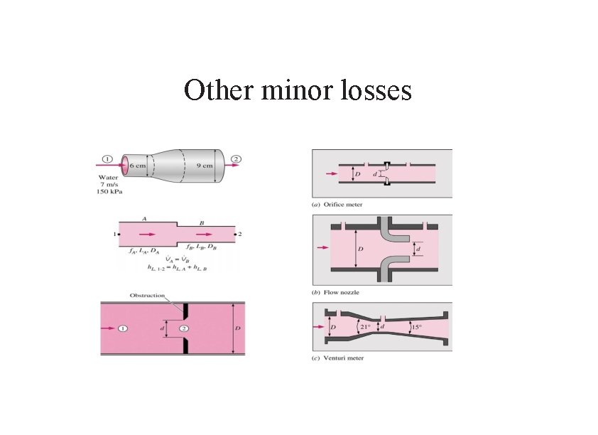
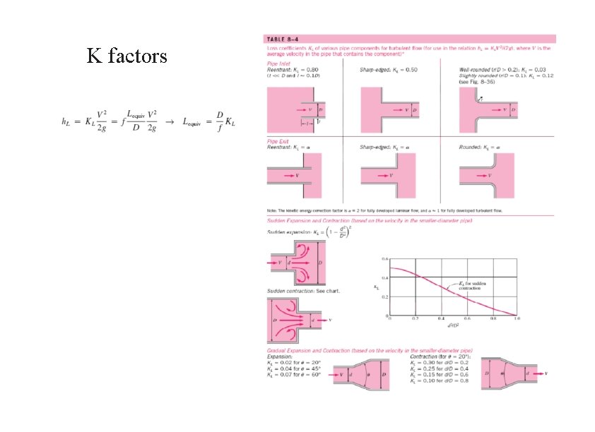
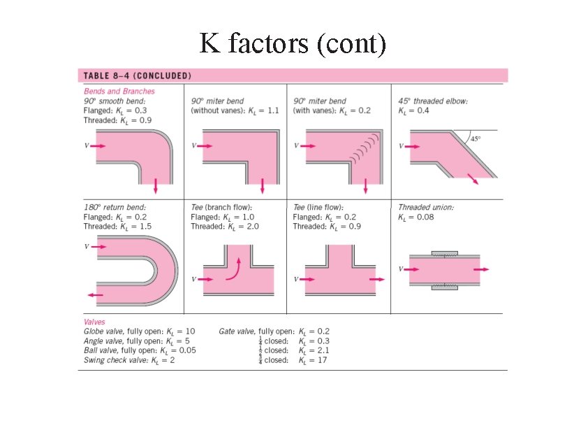
Minor losses The fluid in a typical piping system passes through various fittings, valves, bends, elbows, tees, inlets, exits, enlargements, and contractions in addition to the pipes. These components interrupt the smooth flow of the fluid and cause additional losses because of the flow separation and mixing they induce. In a typical system with long pipes, these losses are minor compared to the total head loss in the pipes (the major losses) and are called minor losses. Although this is generally true, in some cases the minor losses may be greater than the major losses. This is the case, for example, in systems with several turns and valves in a short distance. The head loss introduced by a completely open valve, for example, may be negligible. But a partially closed valve may cause the largest head loss in the system, as evidenced by the drop in the flow rate. Flow through valves and fittings is very complex, and a theoretical analysis is generally not plausible. Therefore, minor losses are determined experimentally, usually by the manufacturers of the components.

Minor losses are usually expressed in terms of the loss coefficient KL (also called the resistance coefficient), defined as Minor losses are also expressed in terms of the equivalent length Lequiv, defined as

Minor losses

Entrance loss

Other minor losses

K factors

K factors (cont)

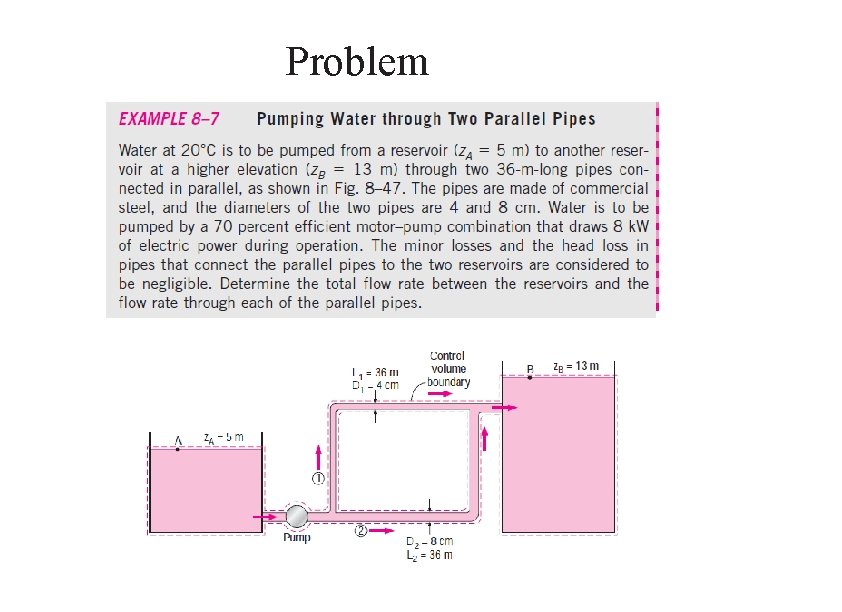
Problem

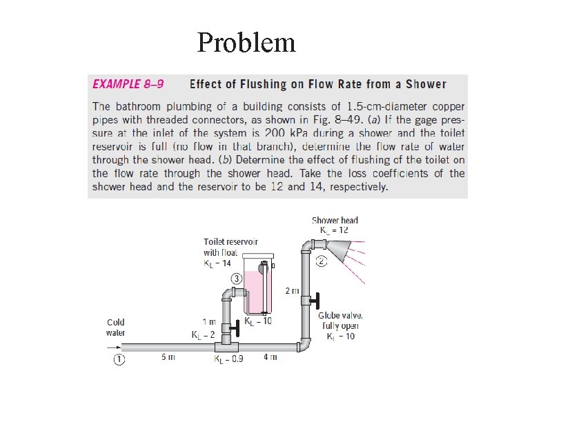
Problem

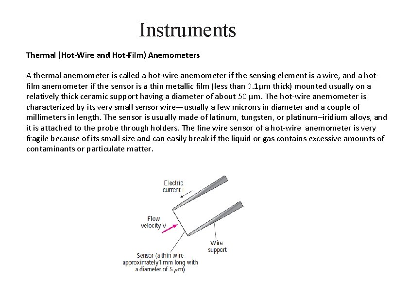
Instruments Thermal (Hot-Wire and Hot-Film) Anemometers A thermal anemometer is called a hot-wire anemometer if the sensing element is a wire, and a hotfilm anemometer if the sensor is a thin metallic film (less than 0. 1μm thick) mounted usually on a relatively thick ceramic support having a diameter of about 50 μm. The hot-wire anemometer is characterized by its very small sensor wire—usually a few microns in diameter and a couple of millimeters in length. The sensor is usually made of latinum, tungsten, or platinum–iridium alloys, and it is attached to the probe through holders. The fine wire sensor of a hot-wire anemometer is very fragile because of its small size and can easily break if the liquid or gas contains excessive amounts of contaminants or particulate matter.

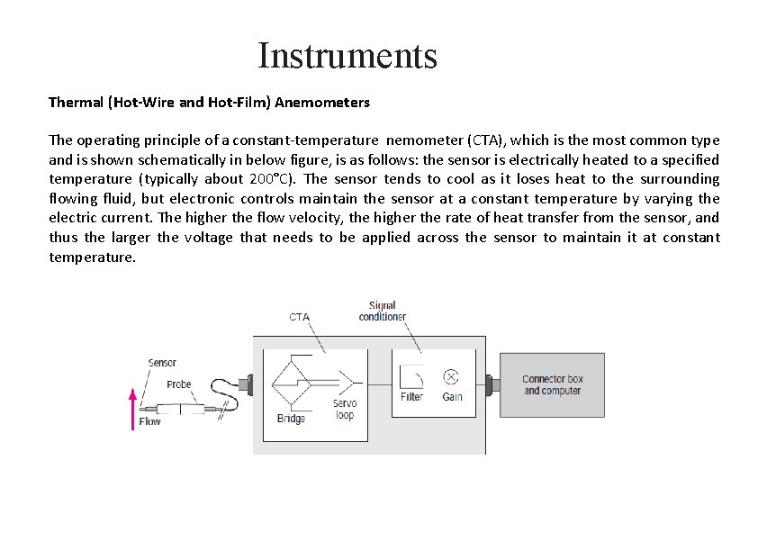
Instruments Thermal (Hot-Wire and Hot-Film) Anemometers The operating principle of a constant-temperature nemometer (CTA), which is the most common type and is shown schematically in below figure, is as follows: the sensor is electrically heated to a specified temperature (typically about 200°C). The sensor tends to cool as it loses heat to the surrounding flowing fluid, but electronic controls maintain the sensor at a constant temperature by varying the electric current. The higher the flow velocity, the higher the rate of heat transfer from the sensor, and thus the larger the voltage that needs to be applied across the sensor to maintain it at constant temperature.

Instruments Thermal (Hot-Wire and Hot-Film) Anemometers The sensor is maintained at a constant temperature during operation, and thus its thermal energy content remains constant. The conservation of energy principle requires that the electrical Joule heating Welectrical = I 2 Rw = E 2/Rw of the sensor must be equal to the total rate of heat loss from the sensor Q total, Using proper relations forced convection, the energy balance can be expressed by King’s law as where a, b and n are constants, they must calibrated by a probe

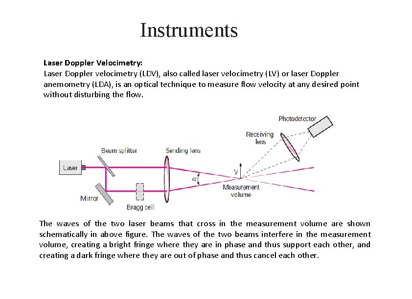
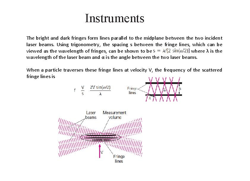
Instruments Laser Doppler Velocimetry: Laser Doppler velocimetry (LDV), also called laser velocimetry (LV) or laser Doppler anemometry (LDA), is an optical technique to measure flow velocity at any desired point without disturbing the flow. The waves of the two laser beams that cross in the measurement volume are shown schematically in above figure. The waves of the two beams interfere in the measurement volume, creating a bright fringe where they are in phase and thus support each other, and creating a dark fringe where they are out of phase and thus cancel each other.

Instruments The bright and dark fringes form lines parallel to the midplane between the two incident laser beams. Using trigonometry, the spacing s between the fringe lines, which can be viewed as the wavelength of fringes, can be shown to be where λ is the wavelength of the laser beam and α is the angle between the two laser beams. When a particle traverses these fringe lines at velocity V, the frequency of the scattered fringe lines is

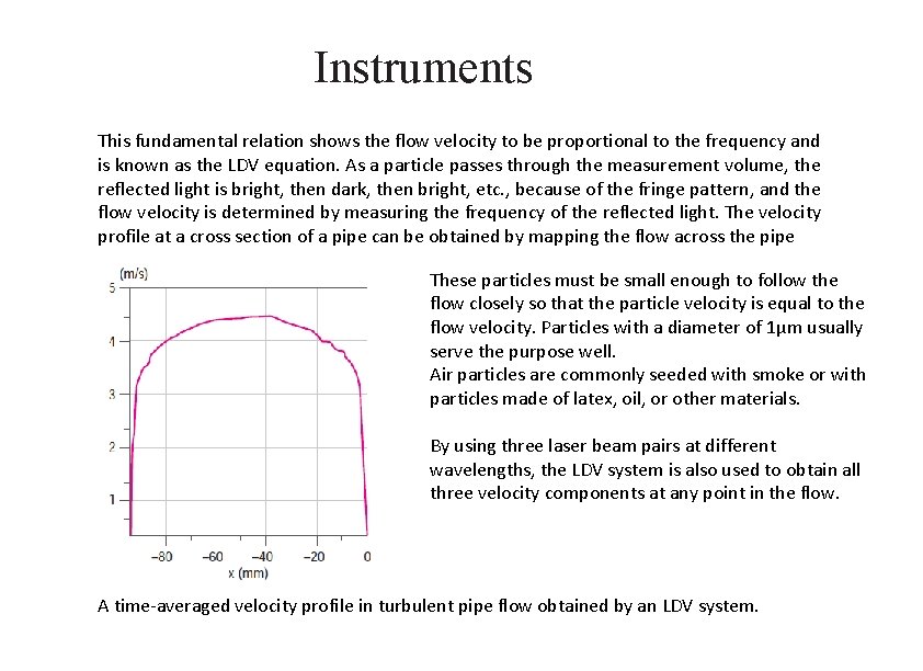
Instruments This fundamental relation shows the flow velocity to be proportional to the frequency and is known as the LDV equation. As a particle passes through the measurement volume, the reflected light is bright, then dark, then bright, etc. , because of the fringe pattern, and the flow velocity is determined by measuring the frequency of the reflected light. The velocity profile at a cross section of a pipe can be obtained by mapping the flow across the pipe These particles must be small enough to follow the flow closely so that the particle velocity is equal to the flow velocity. Particles with a diameter of 1μm usually serve the purpose well. Air particles are commonly seeded with smoke or with particles made of latex, oil, or other materials. By using three laser beam pairs at different wavelengths, the LDV system is also used to obtain all three velocity components at any point in the flow. A time-averaged velocity profile in turbulent pipe flow obtained by an LDV system.

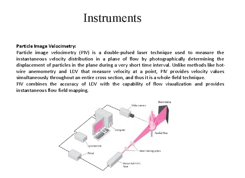
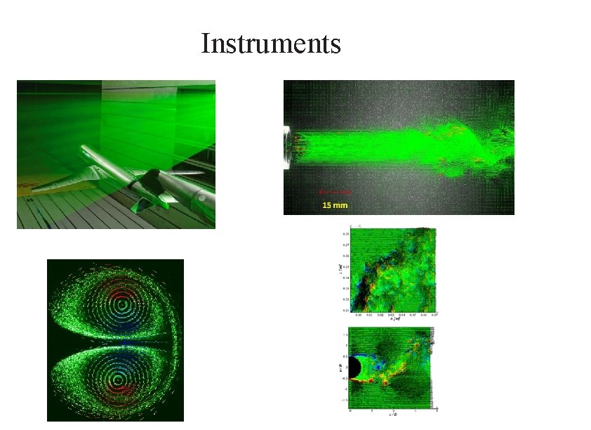
Instruments Particle Image Velocimetry: Particle image velocimetry (PIV) is a double-pulsed laser technique used to measure the instantaneous velocity distribution in a plane of flow by photographically determining the displacement of particles in the plane during a very short time interval. Unlike methods like hotwire anemometry and LDV that measure velocity at a point, PIV provides velocity values simultaneously throughout an entire cross section, and thus it is a whole-field technique. PIV combines the accuracy of LDV with the capability of flow visualization and provides instantaneous flow field mapping.

Instruments Particle Image Velocimetry: A PIV system can be viewed as a camera that can take a snapshot of velocity distribution at any desired plane in a flow. Ordinary flow visualization gives a qualitative picture of the details of flow. PIV is also used to validate computational fluid dynamics (CFD) codes Consists of two main steps: visualization and image processing. Seed the flow with suitable particles in order to trace the fluid motion. Then a pulse of laser light sheet illuminates a thin slice of the flow field at the desired plane, and the positions of particles in that plane are determined by detecting the light scattered by particles on a digital video or photographic camera positioned at right angles to the light sheet. After a very short time period, the particles are illuminated again by a second pulse of laser light sheet, and their new positions are recorded.

Instruments

END