Virtual COMSATS Inferential Statistics Lecture13 Ossam Chohan Assistant

Virtual COMSATS Inferential Statistics Lecture-13 Ossam Chohan Assistant Professor CIIT Abbottabad 1

Recap of previous lecture • • In previous lecture we discussed Two population concepts Independence and Random CI Construction for two cases 2

Objective of this lecture After completing this lecture, you should be able to: • Interval Estimate for – Two independent population means. • Standard deviations known • Standard deviations unknown, but sample sizes>30 • Standard deviations unknown but ni<30 – Two means from paired samples. – The difference between two population proportions.

Population variances are unknown but can be assumed to be equal (t is used) • If it can be assumed that the population variances are equal then each sample variance is actually a point estimate of the same quantity. Therefore, we can combine the sample variances to form a pooled estimate. • Weighted averages The pooled estimated of the common variance is made using weighted averages. This means that each sample variance is weighted by its degrees of freedom. 4

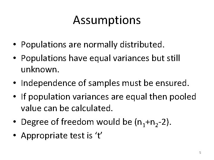
Assumptions • Populations are normally distributed. • Populations have equal variances but still unknown. • Independence of samples must be ensured. • If population variances are equal then pooled value can be calculated. • Degree of freedom would be (n 1+n 2 -2). • Appropriate test is ‘t’ 5

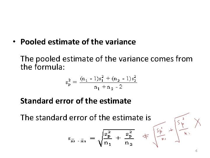
• Pooled estimate of the variance The pooled estimate of the variance comes from the formula: Standard error of the estimate The standard error of the estimate is 6

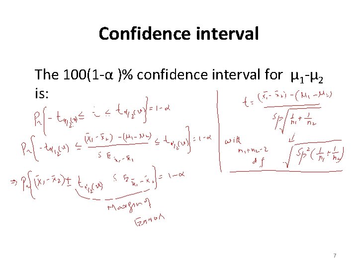
Confidence interval The 100(1 -α )% confidence interval for µ 1 -µ 2 is: 7

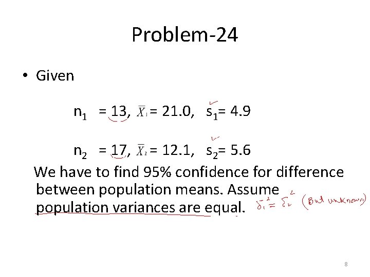
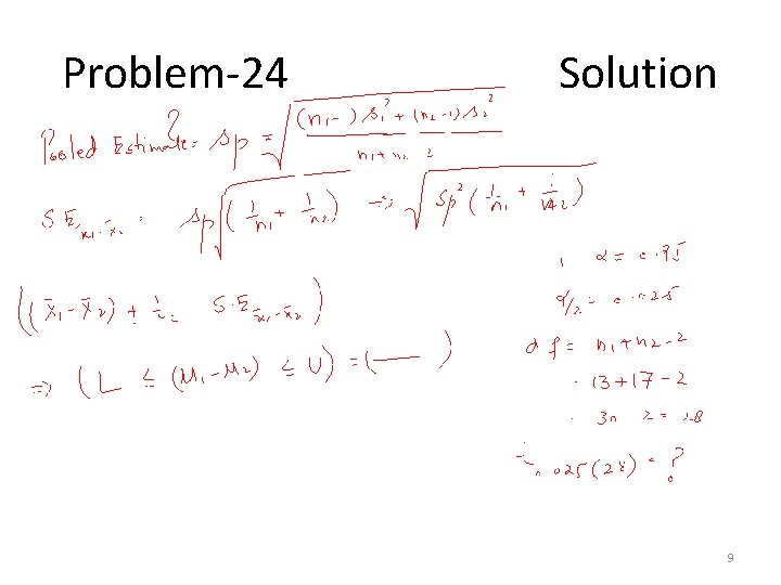
Problem-24 • Given n 1 = 13, = 21. 0, s 1= 4. 9 n 2 = 17, = 12. 1, s 2= 5. 6 We have to find 95% confidence for difference between population means. Assume population variances are equal. 8

Problem-24 Solution 9

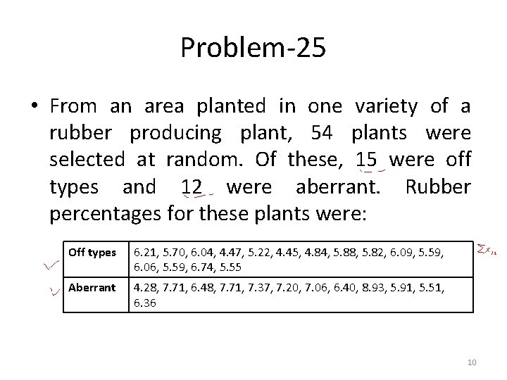
Problem-25 • From an area planted in one variety of a rubber producing plant, 54 plants were selected at random. Of these, 15 were off types and 12 were aberrant. Rubber percentages for these plants were: Off types 6. 21, 5. 70, 6. 04, 4. 47, 5. 22, 4. 45, 4. 84, 5. 88, 5. 82, 6. 09, 5. 59, 6. 06, 5. 59, 6. 74, 5. 55 Aberrant 4. 28, 7. 71, 6. 48, 7. 71, 7. 37, 7. 20, 7. 06, 6. 40, 8. 93, 5. 91, 5. 51, 6. 36 10

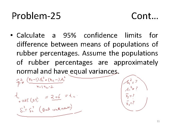
Problem-25 Cont… • Calculate a 95% confidence limits for difference between means of populations of rubber percentages. Assume the populations of rubber percentages are approximately normal and have equal variances. 11

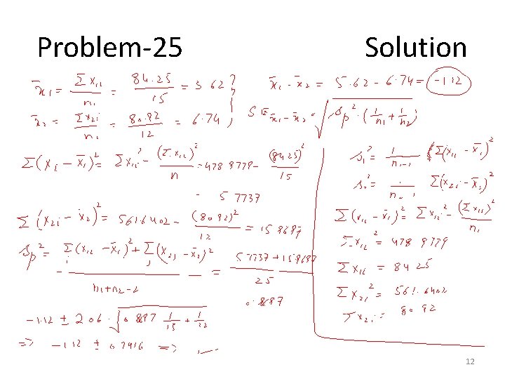
Problem-25 Solution 12

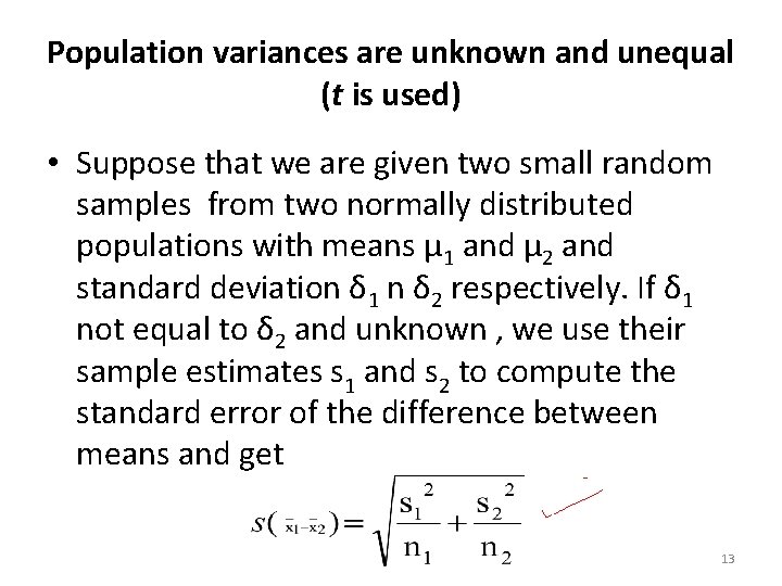
Population variances are unknown and unequal (t is used) • Suppose that we are given two small random samples from two normally distributed populations with means µ 1 and µ 2 and standard deviation δ 1 n δ 2 respectively. If δ 1 not equal to δ 2 and unknown , we use their sample estimates s 1 and s 2 to compute the standard error of the difference between means and get 13

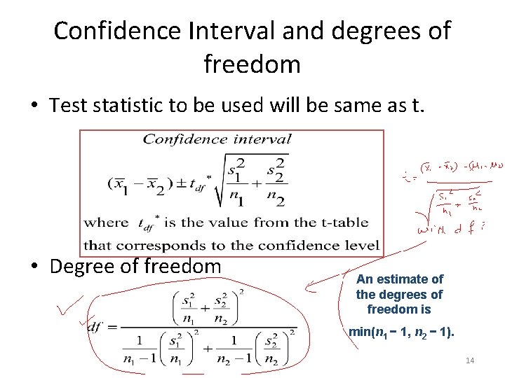
Confidence Interval and degrees of freedom • Test statistic to be used will be same as t. • Degree of freedom An estimate of the degrees of freedom is min(n 1 − 1, n 2 − 1). 14

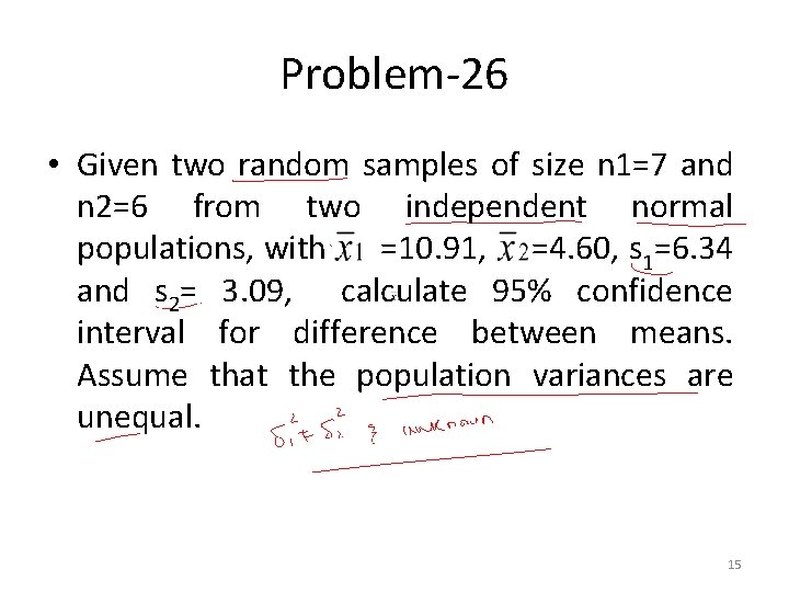
Problem-26 • Given two random samples of size n 1=7 and n 2=6 from two independent normal populations, with =10. 91, =4. 60, s 1=6. 34 and s 2= 3. 09, calculate 95% confidence interval for difference between means. Assume that the population variances are unequal. 15

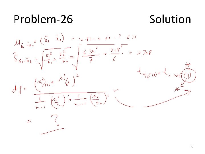
Problem-26 Solution 16

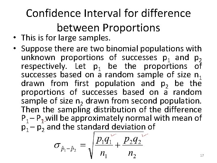
Confidence Interval for difference between Proportions • This is for large samples. • Suppose there are two binomial populations with unknown proportions of successes p 1 and p 2 respectively. Let p 1 be the proportions of successes based on a random sample of size n 1 drawn from first population and p 2 be the proportions of successes based on a random sample of size n 2 drawn from second population. Then the sampling distribution of the difference P 1 – P 1 will be approximately normal with mean of p 1 – p 2 and the standard deviation of 17

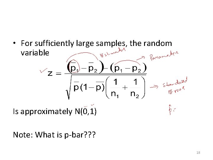
• For sufficiently large samples, the random variable Is approximately N(0, 1) Note: What is p-bar? ? ? 18

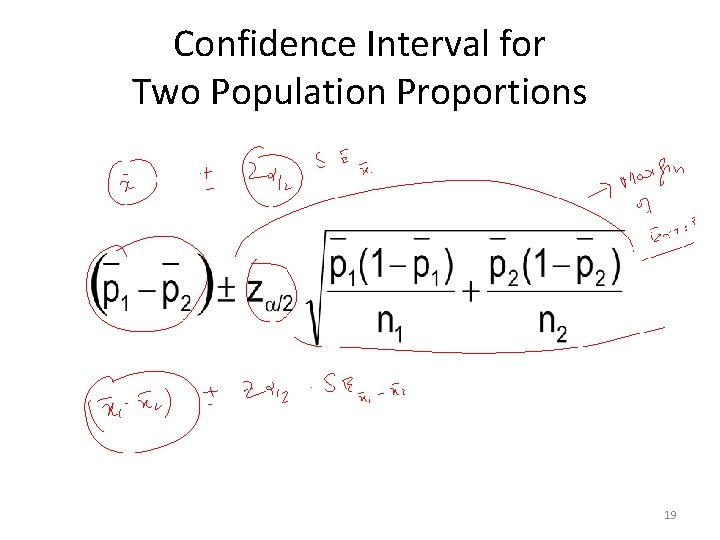
Confidence Interval for Two Population Proportions 19

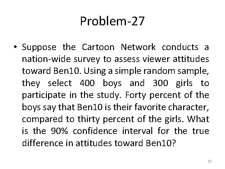
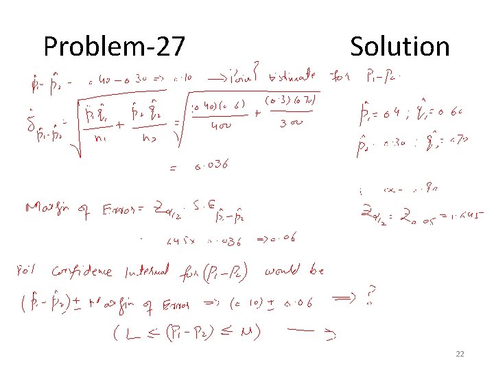
Problem-27 • Suppose the Cartoon Network conducts a nation-wide survey to assess viewer attitudes toward Ben 10. Using a simple random sample, they select 400 boys and 300 girls to participate in the study. Forty percent of the boys say that Ben 10 is their favorite character, compared to thirty percent of the girls. What is the 90% confidence interval for the true difference in attitudes toward Ben 10? 20

Problem-27 Discussion • The sampling method must be simple random sampling. This condition is satisfied; the problem statement says that we used simple random sampling. • Both samples should be independent. This condition is satisfied since neither sample was affected by responses of the other sample. • The sampling distribution should be approximately normally distributed. Because each sample size is large, we know from the central limit theorem that the sampling distribution of the difference between sample proportions will be normal or nearly normal; so this condition is satisfied. 21

Problem-27 Solution 22

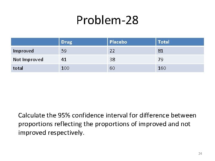
Problem-28 • To study the effectiveness of a drug for some disease, two samples of patients were randomly selected. One sample of 100 was injected with the drug, the other sample of 60 receiving a placebo injection. After a period of time the patients were asked if their disease condition had improved. Results were: 23

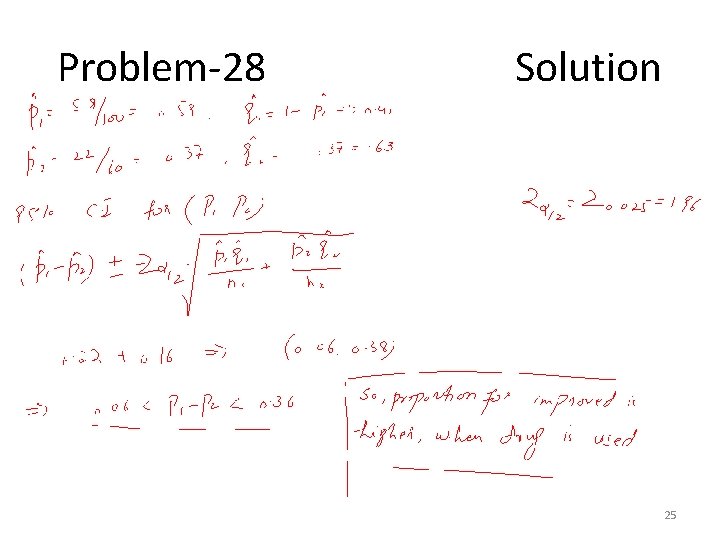
Problem-28 Drug Placebo Total Improved 59 22 81 Not Improved 41 38 79 total 100 60 160 Calculate the 95% confidence interval for difference between proportions reflecting the proportions of improved and not improved respectively. 24

Problem-28 Solution 25

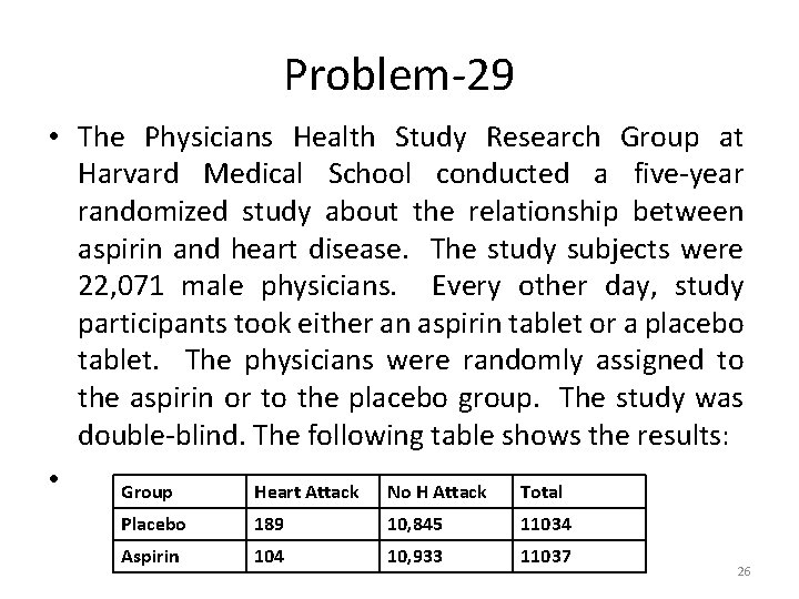
Problem-29 • The Physicians Health Study Research Group at Harvard Medical School conducted a five-year randomized study about the relationship between aspirin and heart disease. The study subjects were 22, 071 male physicians. Every other day, study participants took either an aspirin tablet or a placebo tablet. The physicians were randomly assigned to the aspirin or to the placebo group. The study was double-blind. The following table shows the results: • Group Heart Attack No H Attack Total Placebo 189 10, 845 11034 Aspirin 104 10, 933 11037 26

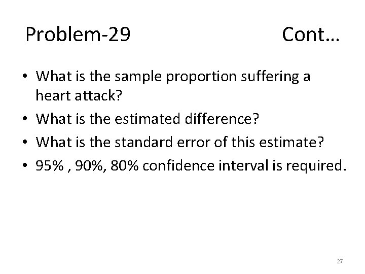
Problem-29 Cont… • What is the sample proportion suffering a heart attack? • What is the estimated difference? • What is the standard error of this estimate? • 95% , 90%, 80% confidence interval is required. 27

Problem-29 Solution 28

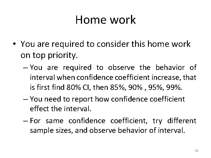
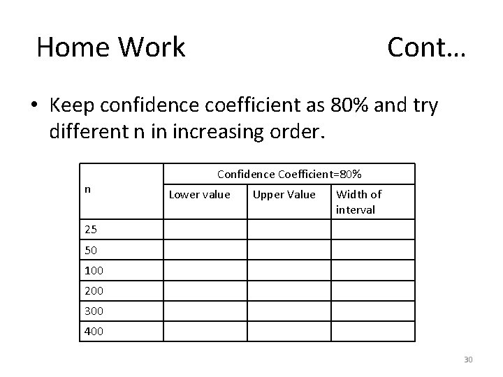
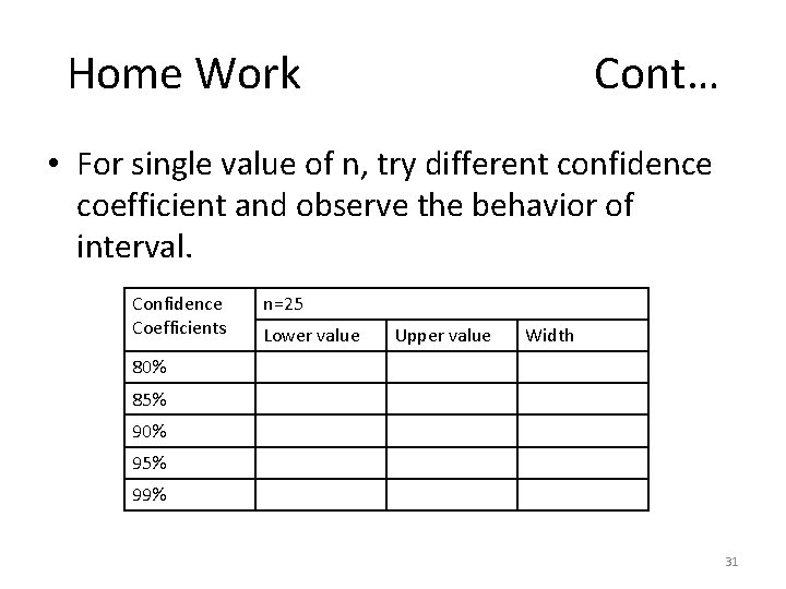
Home work • You are required to consider this home work on top priority. – You are required to observe the behavior of interval when confidence coefficient increase, that is first find 80% CI, then 85%, 90% , 95%, 99%. – You need to report how confidence coefficient effect the interval. – For same confidence coefficient, try different sample sizes, and observe behavior of interval. 29

Home Work Cont… • Keep confidence coefficient as 80% and try different n in increasing order. n Confidence Coefficient=80% Lower value Upper Value Width of interval 25 50 100 200 300 400 30

Home Work Cont… • For single value of n, try different confidence coefficient and observe the behavior of interval. Confidence Coefficients n=25 Lower value Upper value Width 80% 85% 90% 95% 99% 31

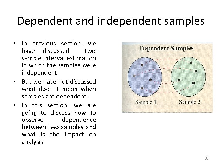
Dependent and independent samples • In previous section, we have discussed twosample interval estimation in which the samples were independent. • But we have not discussed what does it mean when samples are dependent. • In this section, we are going to discuss how to observe dependence between two samples and what is the impact on analysis. 32

Dependent samples? ? ? • Two samples are independent if the sample selected from one population having no relation or impact on the selection (observation) with other sample. • The two samples are dependent if each member of one sample corresponds to a member of the other sample. • Dependent samples are also called paired samples or matched samples. 33

Independent and Dependent Samples • Classify each pair of samples as independent or dependent: Sample 1: Resting heart rates of 35 individuals before drinking coffee. Sample 2: Resting heart rates of the same individuals after drinking two cups of coffee. 34

• These samples are dependent. Because each reading or observation is based on previous result that is before coffee and after coffee. • These samples are related. • The samples can be paired with respect to each individual. 35

Independent and Dependent Samples • Classify each pair of samples as independent or dependent: Sample 1: Test scores for 35 statistics students Sample 2: Test scores for 42 biology students who do not study statistics • What do u think now about independence or dependence? ? ? 36

Important Tip • We can observe that in dependent samples experimental units or subjects are same. • That is for each experimental unit, two observations are recorded. • It means that observation after some experiment will depend upon the previous history. 37

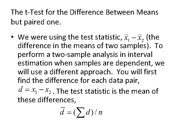
The t-Test for the Difference Between Means but paired one. • We were using the test statistic, (the difference in the means of two samples). To perform a two-sample analysis in interval estimation when samples are dependent, we will use a different approach. You will first find the difference for each data pair, . The test statistic is the mean of these differences,

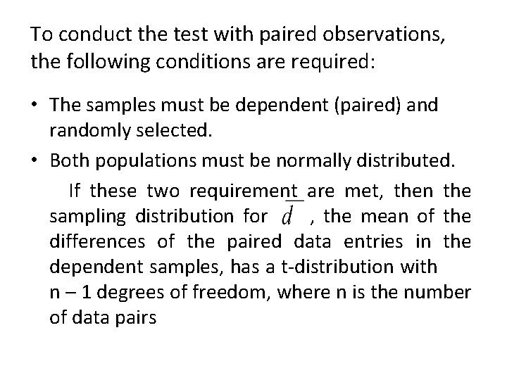
To conduct the test with paired observations, the following conditions are required: • The samples must be dependent (paired) and randomly selected. • Both populations must be normally distributed. If these two requirement are met, then the sampling distribution for , the mean of the differences of the paired data entries in the dependent samples, has a t-distribution with n – 1 degrees of freedom, where n is the number of data pairs

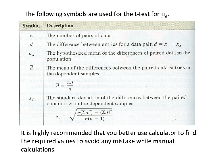
The following symbols are used for the t-test for d. It is highly recommended that you better use calculator to find the required values to avoid any mistake while manual calculations.

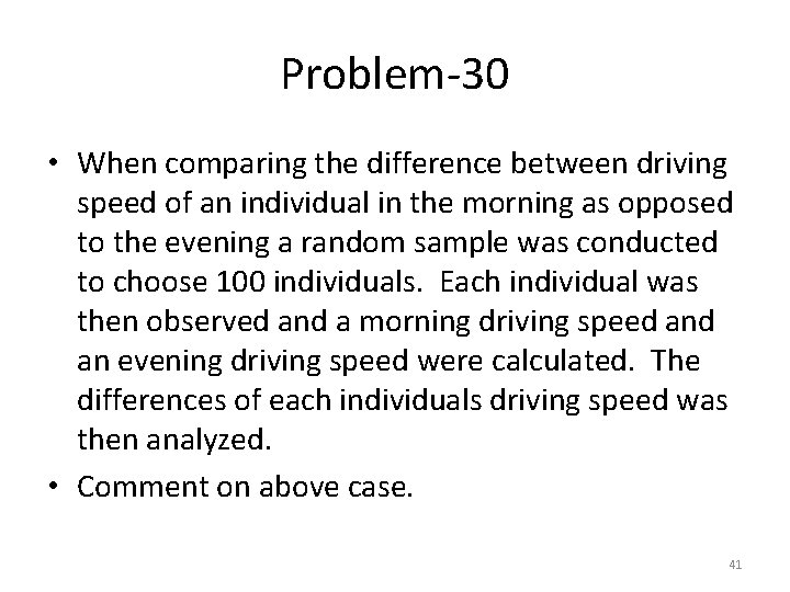
Problem-30 • When comparing the difference between driving speed of an individual in the morning as opposed to the evening a random sample was conducted to choose 100 individuals. Each individual was then observed and a morning driving speed an evening driving speed were calculated. The differences of each individuals driving speed was then analyzed. • Comment on above case. 41

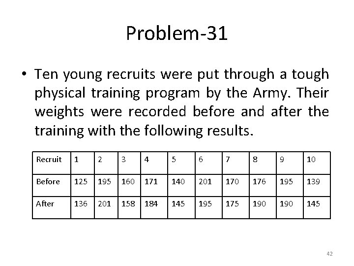
Problem-31 • Ten young recruits were put through a tough physical training program by the Army. Their weights were recorded before and after the training with the following results. Recruit 1 2 3 4 5 6 7 8 9 10 Before 125 195 160 171 140 201 170 176 195 139 After 136 201 158 184 145 195 175 190 145 42

Problem-31 Cont… • Analyze the problem and check either it is dependent case or independent? • Construct 95% confidence interval for efficiency of program with respect to weight. 43

Problem-31 Solution 44

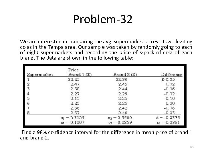
Problem-32 We are interested in comparing the avg. supermarket prices of two leading colas in the Tampa area. Our sample was taken by randomly going to each of eight supermarkets and recording the price of s-pack of cola of each brand. The data are shown in the following table: Find a 98% confidence interval for the difference in mean price of brand 1 and brand 2. 45

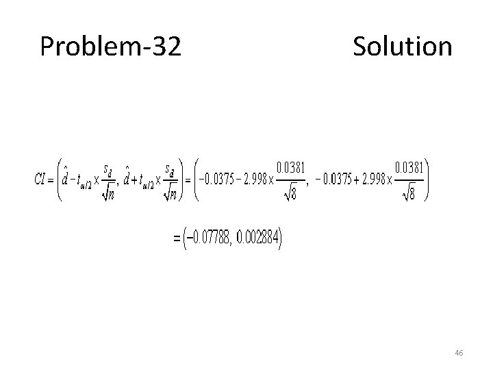
Problem-32 Solution 46

One sided confidence interval • So far we have studied two sided 100(1 -α)% confidence interval. • Because interval specified both lower and upper limits of any particular parameter. • We may wish to have only one tail (limit). • Therefore α area will be located at one side of the sampling distribution. 47

Problem-32 • For estimating the average weight of college students in Lahore city, a sample of 100 college students is randomly selected and a sample mean of 120 pounds is obtained. Assume that the variance of the population is 1600. determine the lower limit of the 95% confidence interval where upper limit is 280 pounds. 48

Problem-32 Solution 49

Practice Problems • In this section, we will go through various problems without having any title and will try to understand the suitable approach to solve problems. • This will include different problems like single mean, proportions, difference between means, proportions, z, t statistics, paired case. 50

Practice Problem-1 • In order to ensure efficient usage of a server, it is necessary to estimate the mean number of concurrent users. According to records, the sample mean and sample standard deviation of number of concurrent users at 100 randomly selected times is 37. 7 and 9. 2, respectively. • Construct a 90% confidence interval for the mean number of concurrent users. 51

Practice Problem-1 Solution 52

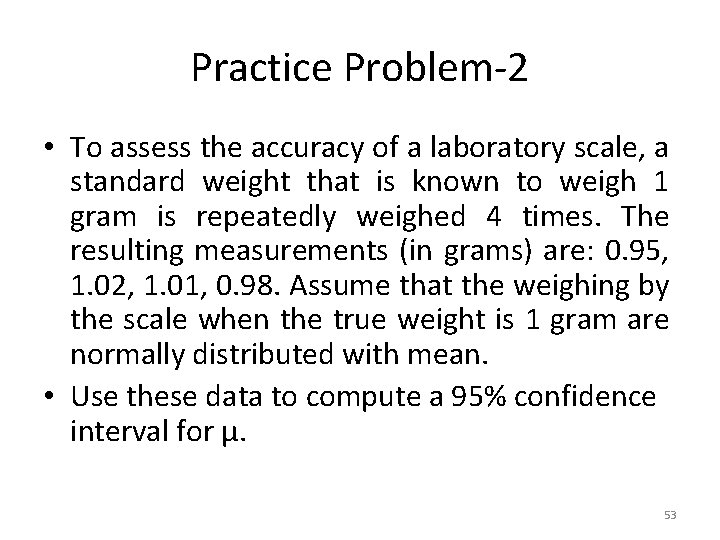
Practice Problem-2 • To assess the accuracy of a laboratory scale, a standard weight that is known to weigh 1 gram is repeatedly weighed 4 times. The resulting measurements (in grams) are: 0. 95, 1. 02, 1. 01, 0. 98. Assume that the weighing by the scale when the true weight is 1 gram are normally distributed with mean. • Use these data to compute a 95% confidence interval for µ. 53

Practice Problem-2 Solution 54

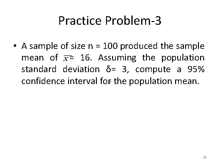
Practice Problem-3 • A sample of size n = 100 produced the sample mean of = 16. Assuming the population standard deviation δ= 3, compute a 95% confidence interval for the population mean. 55

Practice Problem-3 Solution 56

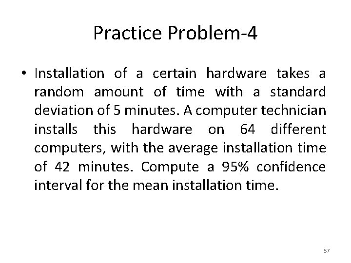
Practice Problem-4 • Installation of a certain hardware takes a random amount of time with a standard deviation of 5 minutes. A computer technician installs this hardware on 64 different computers, with the average installation time of 42 minutes. Compute a 95% confidence interval for the mean installation time. 57

Practice Problem-4 Solution 58

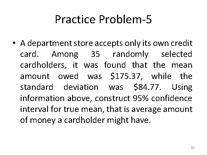
Practice Problem-5 • A department store accepts only its own credit card. Among 35 randomly selected cardholders, it was found that the mean amount owed was $175. 37, while the standard deviation was $84. 77. Using information above, construct 95% confidence interval for true mean, that is average amount of money a cardholder might have. 59

Practice Problem-5 Solution 60

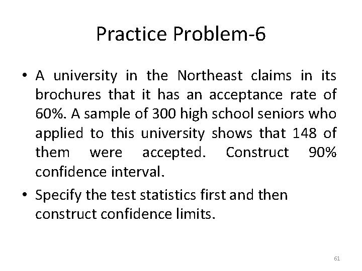
Practice Problem-6 • A university in the Northeast claims in its brochures that it has an acceptance rate of 60%. A sample of 300 high school seniors who applied to this university shows that 148 of them were accepted. Construct 90% confidence interval. • Specify the test statistics first and then construct confidence limits. 61

Practice problem-6 Solution 62

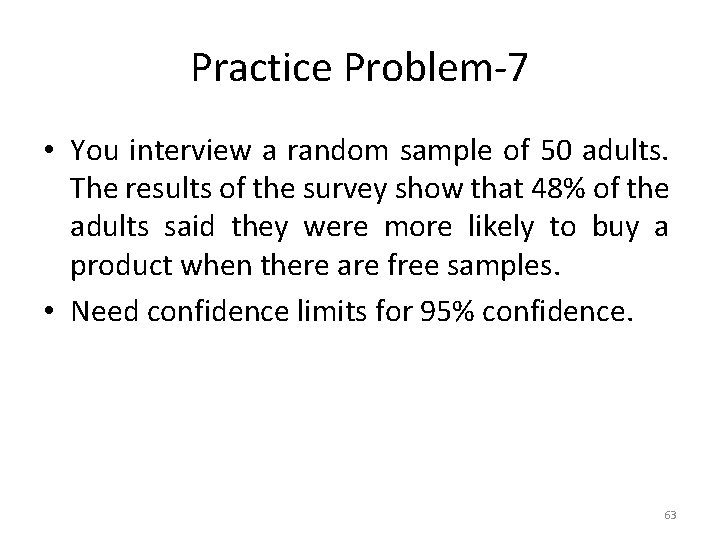
Practice Problem-7 • You interview a random sample of 50 adults. The results of the survey show that 48% of the adults said they were more likely to buy a product when there are free samples. • Need confidence limits for 95% confidence. 63

Practice Problem-7 Solution 64

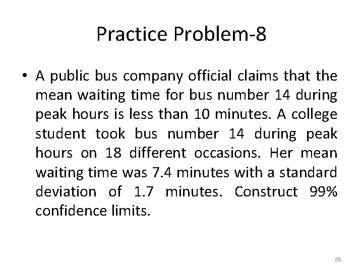
Practice Problem-8 • A public bus company official claims that the mean waiting time for bus number 14 during peak hours is less than 10 minutes. A college student took bus number 14 during peak hours on 18 different occasions. Her mean waiting time was 7. 4 minutes with a standard deviation of 1. 7 minutes. Construct 99% confidence limits. 65

Practice Problem-8 Solution 66

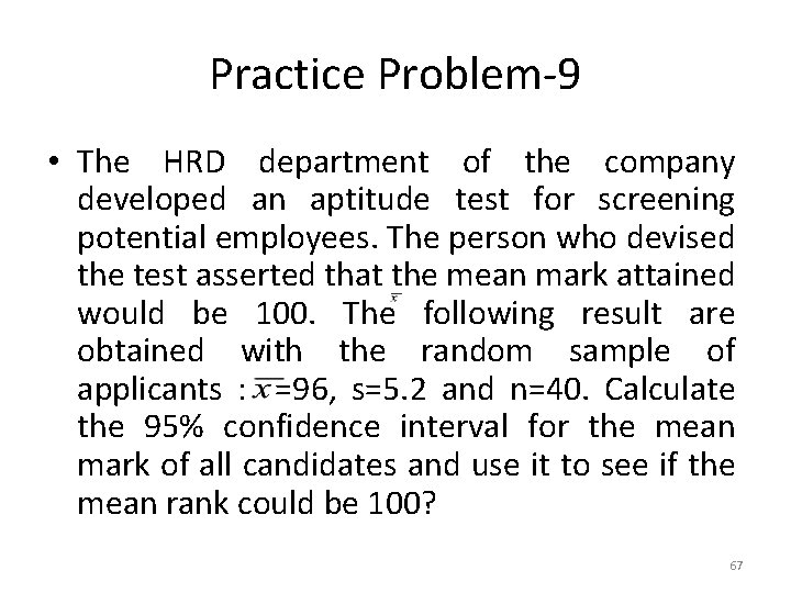
Practice Problem-9 • The HRD department of the company developed an aptitude test for screening potential employees. The person who devised the test asserted that the mean mark attained would be 100. The following result are obtained with the random sample of applicants : =96, s=5. 2 and n=40. Calculate the 95% confidence interval for the mean mark of all candidates and use it to see if the mean rank could be 100? 67

Practice Problem-9 Solution 68

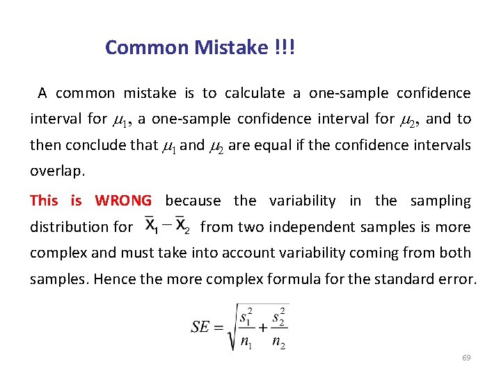
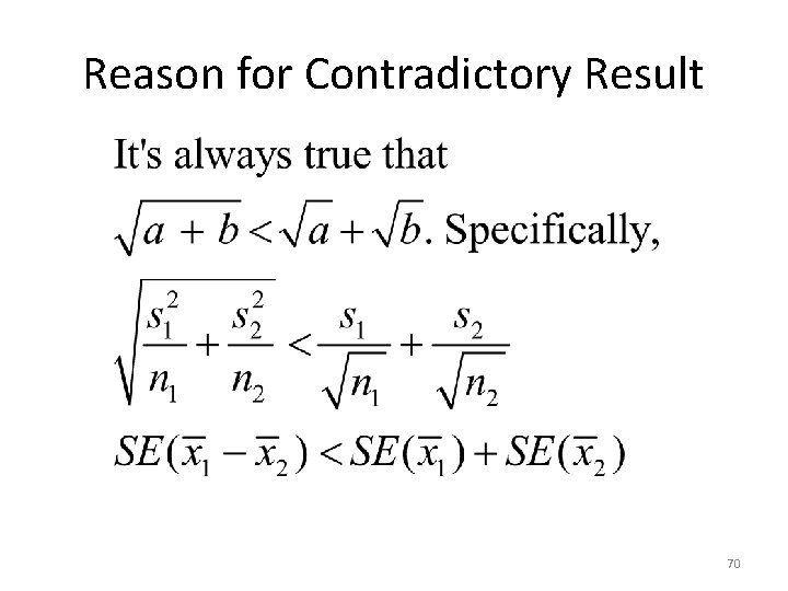
Common Mistake !!! A common mistake is to calculate a one-sample confidence interval for m 1, a one-sample confidence interval for m 2, and to then conclude that m 1 and m 2 are equal if the confidence intervals overlap. This is WRONG because the variability in the sampling distribution for from two independent samples is more complex and must take into account variability coming from both samples. Hence the more complex formula for the standard error. 69

Reason for Contradictory Result 70

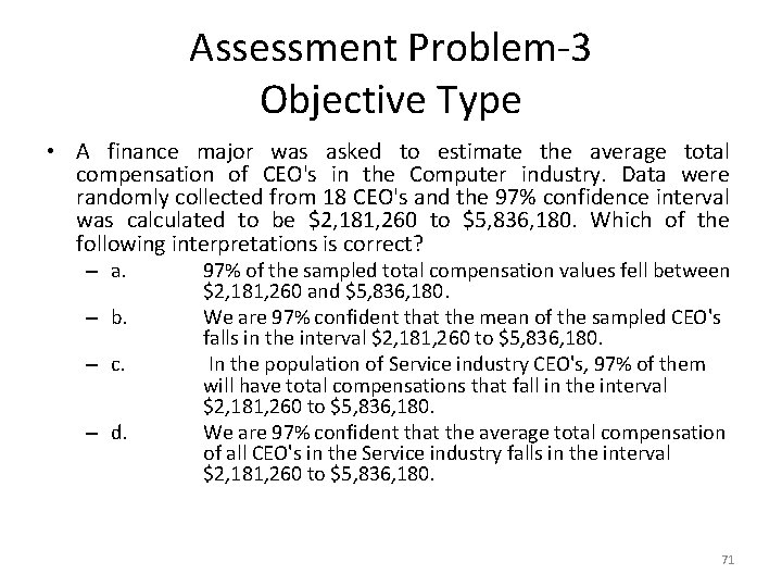
Assessment Problem-3 Objective Type • A finance major was asked to estimate the average total compensation of CEO's in the Computer industry. Data were randomly collected from 18 CEO's and the 97% confidence interval was calculated to be $2, 181, 260 to $5, 836, 180. Which of the following interpretations is correct? – a. – b. – c. – d. 97% of the sampled total compensation values fell between $2, 181, 260 and $5, 836, 180. We are 97% confident that the mean of the sampled CEO's falls in the interval $2, 181, 260 to $5, 836, 180. In the population of Service industry CEO's, 97% of them will have total compensations that fall in the interval $2, 181, 260 to $5, 836, 180. We are 97% confident that the average total compensation of all CEO's in the Service industry falls in the interval $2, 181, 260 to $5, 836, 180. 71

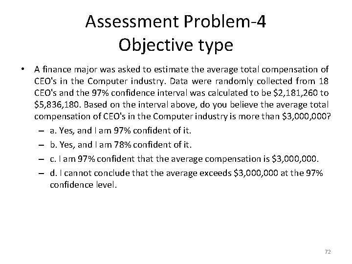
Assessment Problem-4 Objective type • A finance major was asked to estimate the average total compensation of CEO's in the Computer industry. Data were randomly collected from 18 CEO's and the 97% confidence interval was calculated to be $2, 181, 260 to $5, 836, 180. Based on the interval above, do you believe the average total compensation of CEO's in the Computer industry is more than $3, 000? – a. Yes, and I am 97% confident of it. – b. Yes, and I am 78% confident of it. – c. I am 97% confident that the average compensation is $3, 000. – d. I cannot conclude that the average exceeds $3, 000 at the 97% confidence level. 72

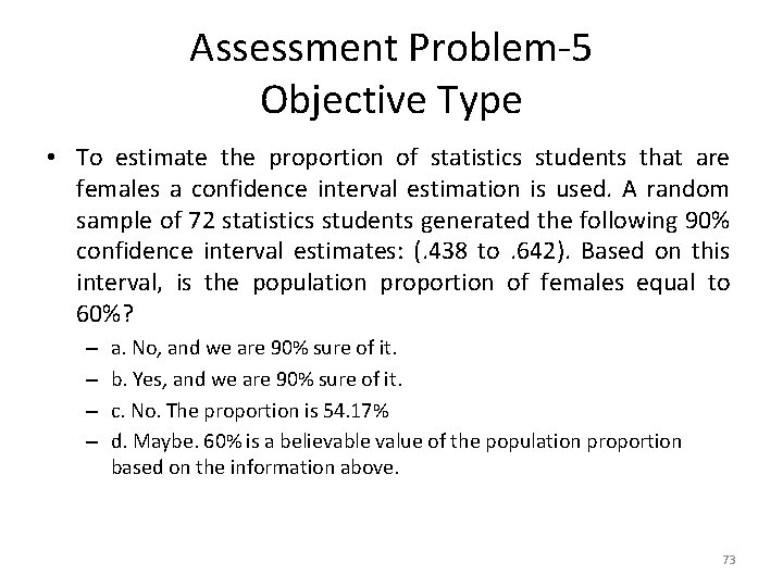
Assessment Problem-5 Objective Type • To estimate the proportion of statistics students that are females a confidence interval estimation is used. A random sample of 72 statistics students generated the following 90% confidence interval estimates: (. 438 to . 642). Based on this interval, is the population proportion of females equal to 60%? – – a. No, and we are 90% sure of it. b. Yes, and we are 90% sure of it. c. No. The proportion is 54. 17% d. Maybe. 60% is a believable value of the population proportion based on the information above. 73

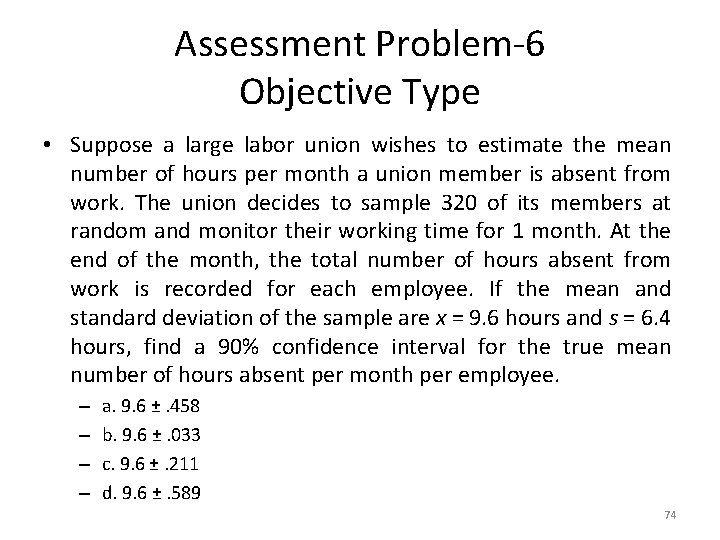
Assessment Problem-6 Objective Type • Suppose a large labor union wishes to estimate the mean number of hours per month a union member is absent from work. The union decides to sample 320 of its members at random and monitor their working time for 1 month. At the end of the month, the total number of hours absent from work is recorded for each employee. If the mean and standard deviation of the sample are x = 9. 6 hours and s = 6. 4 hours, find a 90% confidence interval for the true mean number of hours absent per month per employee. – – a. 9. 6 ±. 458 b. 9. 6 ±. 033 c. 9. 6 ±. 211 d. 9. 6 ±. 589 74

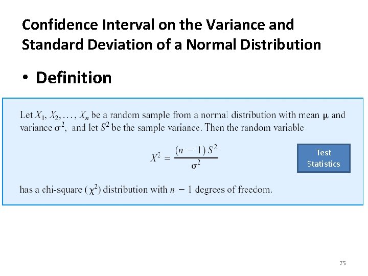
Confidence Interval on the Variance and Standard Deviation of a Normal Distribution • Definition Test Statistics 75

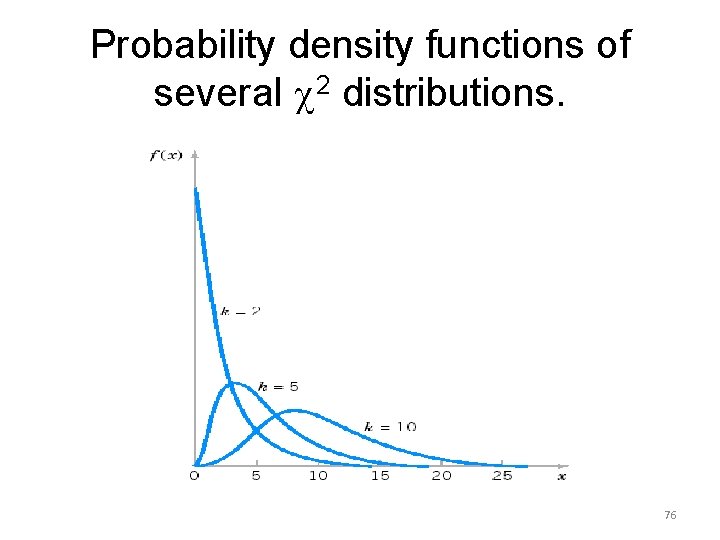
Probability density functions of several 2 distributions. 76

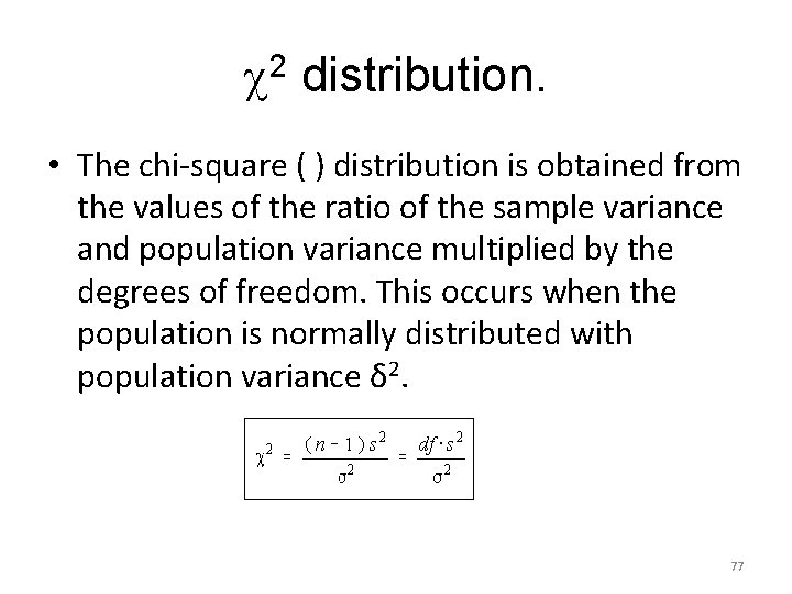
2 distribution. • The chi-square ( ) distribution is obtained from the values of the ratio of the sample variance and population variance multiplied by the degrees of freedom. This occurs when the population is normally distributed with population variance δ 2. 77

Properties and Characteristics: • Chi-square density curves are right-skewed. • Each Chi-square random variable is associated with a degree of freedom (υ), . As υ increase, Chi-square curves become more symmetric. • Z 2, the square of a normal[0, 1] random variable, follows a Chi square (with 1 df)distribution. • Chi-square is non-negative and the ratio of two nonnegative values, therefore must be non-negative itself. • Chi-square is non-symmetric • There are many different chi-square distributions, one for each degree of freedom. • The degrees of freedom when working with a single population variance is n-1. 78

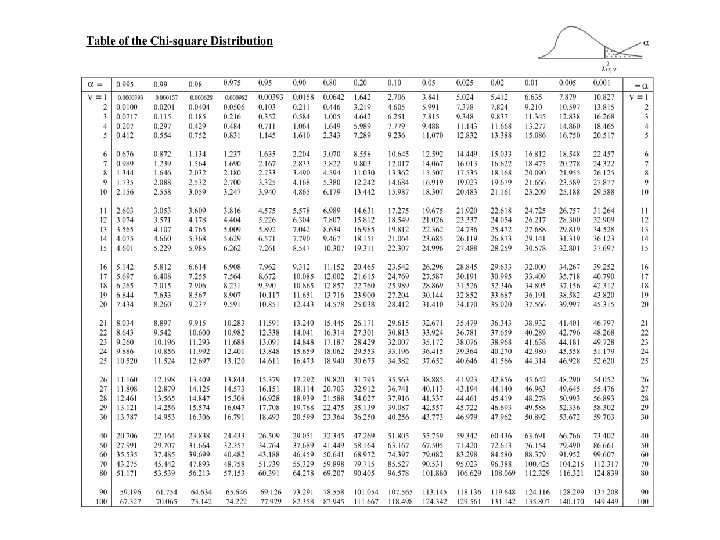
Confidence Interval construction for population variance. 79

Can we find CI for population standard deviation? ? 80

81

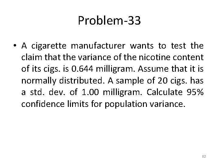
Problem-33 • A cigarette manufacturer wants to test the claim that the variance of the nicotine content of its cigs. is 0. 644 milligram. Assume that it is normally distributed. A sample of 20 cigs. has a std. dev. of 1. 00 milligram. Calculate 95% confidence limits for population variance. 82

Problem-33 Solution 83

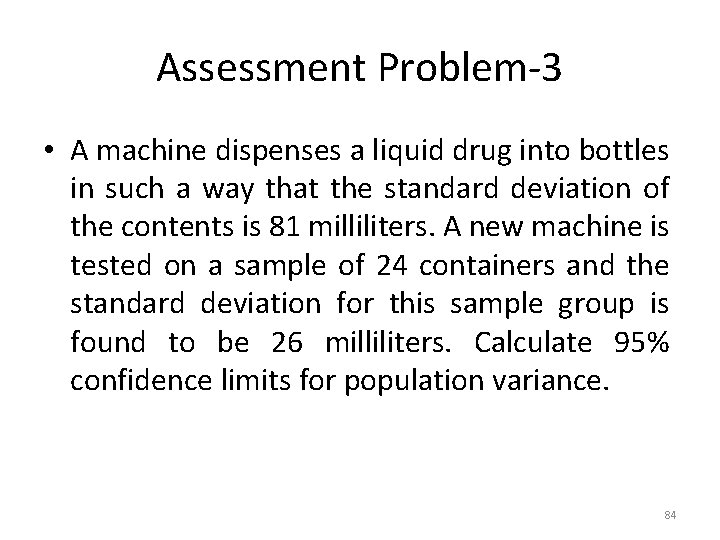
Assessment Problem-3 • A machine dispenses a liquid drug into bottles in such a way that the standard deviation of the contents is 81 milliliters. A new machine is tested on a sample of 24 containers and the standard deviation for this sample group is found to be 26 milliliters. Calculate 95% confidence limits for population variance. 84

Assessment Problem Discussion 85

Introduction to Hypothesis Testing 86

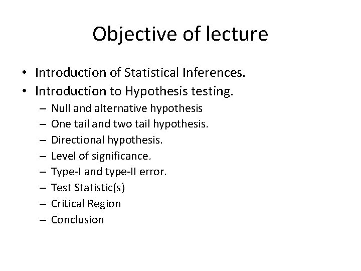
Objective of lecture • Introduction of Statistical Inferences. • Introduction to Hypothesis testing. – – – – Null and alternative hypothesis One tail and two tail hypothesis. Directional hypothesis. Level of significance. Type-I and type-II error. Test Statistic(s) Critical Region Conclusion

Introduction • “Hypothesis testing can be defined as an inferential procedure that uses sample data to evaluate the credibility of a hypothesis about a population” • Hypothesis: – “A tentative statement about a population parameter that might be true or wrong” – Why Hypothesis?

• A hypothesis is an assumption about the population parameter. – – A parameter is a Population mean or proportion or any other characteristics of population The parameter must be identified before analysis. • A hypothesis is a specific, testable prediction about what you expect to happen in your study.

Examples of Hypotheses • An operation manager wants to determine if the mean demand during lead time is greater than 350. • Assume that population mean age is 50. • More students get sick during the final week of testing that at other times. • Amount of sun exposure will increase the growth of a tomato plant. • There is a positive correlation between the availability of hours for work and the productivity of employees. • Worker satisfaction increases worker productivity.

Basics About Hypotheses The two types of hypotheses are scientific and working. • A scientific hypothesis is based on experiments and observations from the past that cannot be explained with current theories. • A working hypothesis is one that is widely accepted and becomes the basis of further experimentation.

Good Hypothesis • In order to be a good hypothesis that can be tested or studied, a hypothesis: – Needs to be logical – Must use precise language – Should be testable with research or experimentation

Hypothesis, Law and Theory • Hypothesis: – A hypothesis will give a plausible explanation that will be tested. It can also explain future phenomenon that will need to be tested. • Law: – Once a hypothesis has been widely accepted, it is called a law. This means that it is assumed to be true and will predict the outcome of certain conditions or experiments. • Theory: – A scientific theory is broader in scope and explains more events that a law. After hypotheses and laws have been tested many times, with accurate results, they become theories.

Finally what is hypothesis? • A statistical hypothesis is a claim (assertion, statement, belief or assumption) about an unknown population parameter value. • For example an investment company claims that the average return across all its investments is 20 percent and so on. To test such claims sample data are collected analyzed. • On the basis of sample findings hypothesized value of population parameter is accepted or rejected. 94

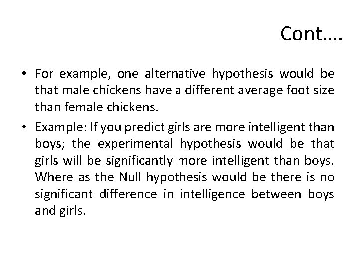
Types of Hypothesis • Null hypothesis: – The null hypothesis is a statement that you want to test. For example, if you measure the size of the feet of male and female chickens, the null hypothesis could be that the average foot size in male chickens is the same as the average foot size in female chickens • Research/ Alternative hypothesis: – The alternative hypothesis is that things are different from each other, or different from a theoretical expectation.

Cont…. • For example, one alternative hypothesis would be that male chickens have a different average foot size than female chickens. • Example: If you predict girls are more intelligent than boys; the experimental hypothesis would be that girls will be significantly more intelligent than boys. Where as the Null hypothesis would be there is no significant difference in intelligence between boys and girls.

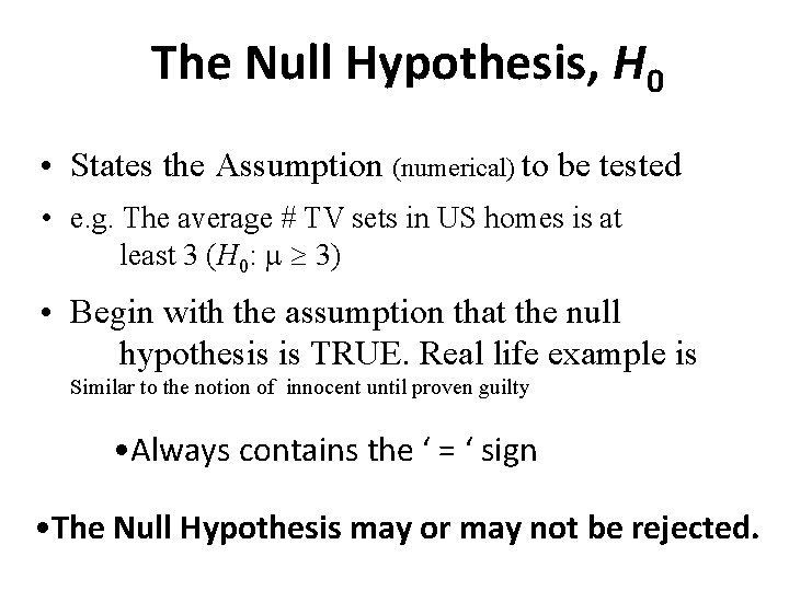
The Null Hypothesis, H 0 • States the Assumption (numerical) to be tested • e. g. The average # TV sets in US homes is at least 3 (H 0: ³ 3) • Begin with the assumption that the null hypothesis is TRUE. Real life example is Similar to the notion of innocent until proven guilty • Always contains the ‘ = ‘ sign • The Null Hypothesis may or may not be rejected.

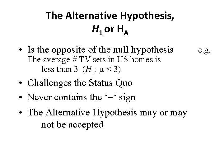
The Alternative Hypothesis, H 1 or HA • Is the opposite of the null hypothesis The average # TV sets in US homes is less than 3 (H 1: < 3) • Challenges the Status Quo • Never contains the ‘=‘ sign • The Alternative Hypothesis may or may not be accepted e. g.

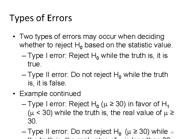
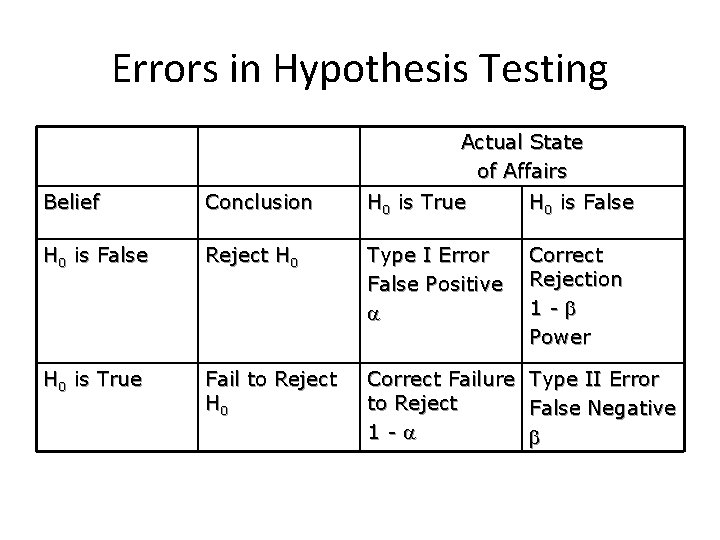
Types of Errors • Two types of errors may occur when deciding whether to reject H 0 based on the statistic value. – Type I error: Reject H 0 while the truth is, it is true. – Type II error: Do not reject H 0 while the truth is, it is false. • Example continued – Type I error: Reject H 0 ( ≥ 30) in favor of H 1 ( < 30) while the truth is, the real value of ≥ 30. – Type II error: Do not reject H 0 ( ≥ 30) while 99

Types of Errors-discussion 100

Errors in Hypothesis Testing Actual State of Affairs Belief Conclusion H 0 is True H 0 is False Reject H 0 Type I Error False Positive Correct Rejection 1 - Power H 0 is True Fail to Reject H 0 Correct Failure to Reject 1 - Type II Error False Negative

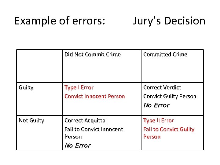
Example of errors: Jury’s Decision Did Not Commit Crime Committed Crime Guilty Type I Error Convict Innocent Person Correct Verdict Convict Guilty Person No Error Not Guilty Correct Acquittal Fail to Convict Innocent Person No Error Type II Error Fail to Convict Guilty Person

Practical Problem for understanding • We will use following example throughout the understanding phase of introduction. And we will add some more problems to make it more clear.

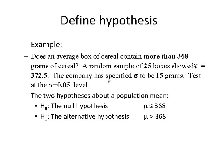
Define hypothesis – Example: – Does an average box of cereal contain more than 368 grams of cereal? A random sample of 25 boxes showed = 372. 5. The company has specified s to be 15 grams. Test at the =0. 05 level. – The two hypotheses about a population mean: • H 0: The null hypothesis ≤ 368 • H 1: The alternative hypothesis > 368

Important Tips • How to represent hypothesis? • Role of equality in hypothesis?

Discussion

Discussion continued

One tail/Two tail hypothesis • Is that example one tail or two tail? Justify

Directional Hypothesis

Level of Significance Alpha: probability of committing a Type I error 1. 2. Reject H 0 although it is true Symbolized by • What about probability of type-II error? • What is the role of type-II error in HT? • Probability that the test will correctly reject a false null hypothesis-Power of the Test 110

• The significance level of a statistical hypothesis test is a fixed probability of wrongly rejecting the null hypothesis H 0, if it is in fact true. It is the probability of a type-I error and is set by the investigator in relation to the consequences of such an error. That is, we want to make the significance level as small as possible in order to protect the null hypothesis and to prevent, as far as possible, the investigator from inadvertently making false claims. • The significance level is usually denoted by significance level = P (type I error) = α • Usually, the significance level is chosen to be 0. 05 (or equivalently, 5%). 111

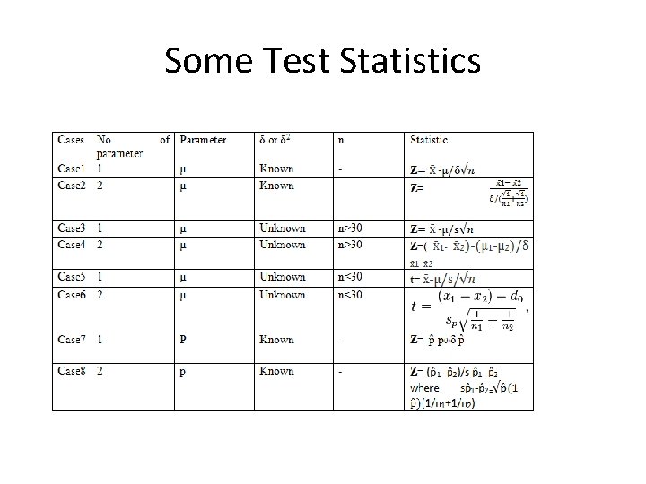
Identifying δ and observe n • The role of population variation and sample size is highly significant in drawing inferencesstatistical, as we discussed in estimation section. • All the rules are same as we discussed in estimation. • Selection of test statistics depends upon population variability and sample size. (obviously CLT plays role here) 112

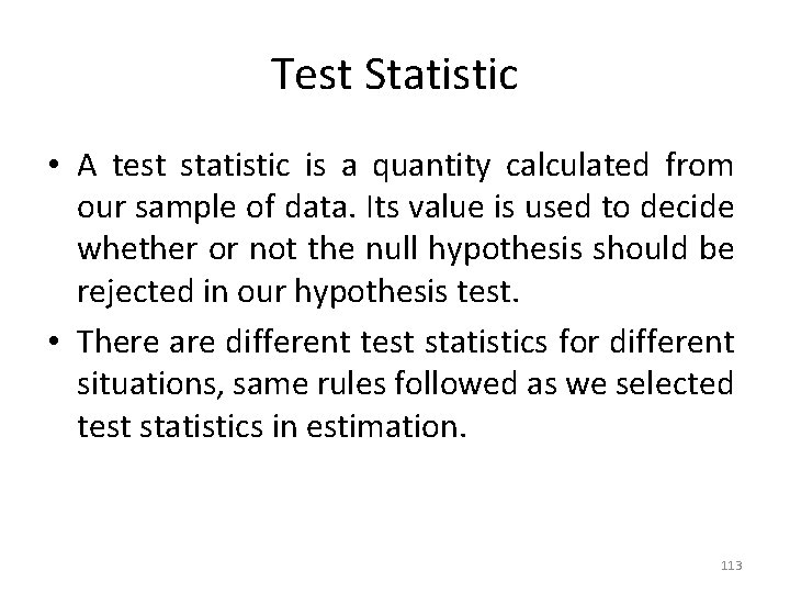
Test Statistic • A test statistic is a quantity calculated from our sample of data. Its value is used to decide whether or not the null hypothesis should be rejected in our hypothesis test. • There are different test statistics for different situations, same rules followed as we selected test statistics in estimation. 113

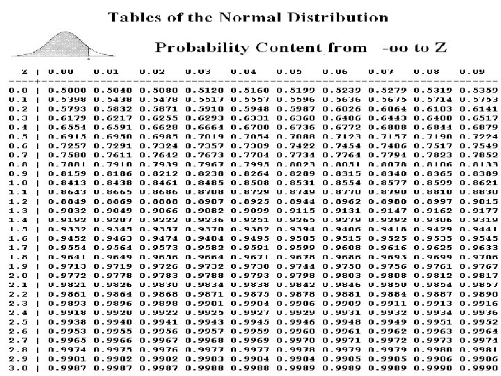
Some Test Statistics 114

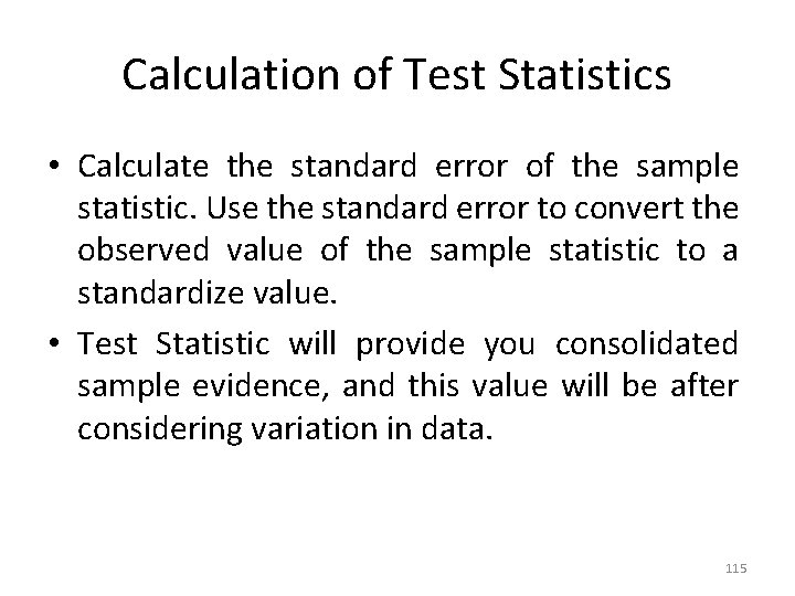
Calculation of Test Statistics • Calculate the standard error of the sample statistic. Use the standard error to convert the observed value of the sample statistic to a standardize value. • Test Statistic will provide you consolidated sample evidence, and this value will be after considering variation in data. 115

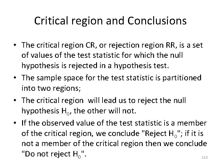
Critical region and Conclusions • The critical region CR, or rejection region RR, is a set of values of the test statistic for which the null hypothesis is rejected in a hypothesis test. • The sample space for the test statistic is partitioned into two regions; • The critical region will lead us to reject the null hypothesis H 0, the other will not. • If the observed value of the test statistic is a member of the critical region, we conclude "Reject H 0"; if it is not a member of the critical region then we conclude "Do not reject H 0". 116

Assessment Problem-3 • We know that the statement • P( -1. 96δ <µ< +1. 96δ )=0. 95 is correct, while the statement P(140<µ<160)=0. 95 is not correct. Explain why the latter is erroneous? • Some guidelines…. 117

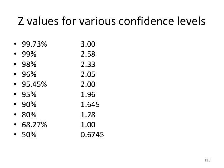
Z values for various confidence levels • • • 99. 73% 99% 98% 96% 95. 45% 90% 80% 68. 27% 50% 3. 00 2. 58 2. 33 2. 05 2. 00 1. 96 1. 645 1. 28 1. 00 0. 6745 118

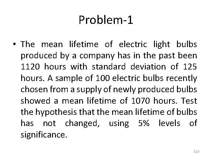
Problem-1 • The mean lifetime of electric light bulbs produced by a company has in the past been 1120 hours with standard deviation of 125 hours. A sample of 100 electric bulbs recently chosen from a supply of newly produced bulbs showed a mean lifetime of 1070 hours. Test the hypothesis that the mean lifetime of bulbs has not changed, using 5% levels of significance. 119

Problem-1 Solution 120

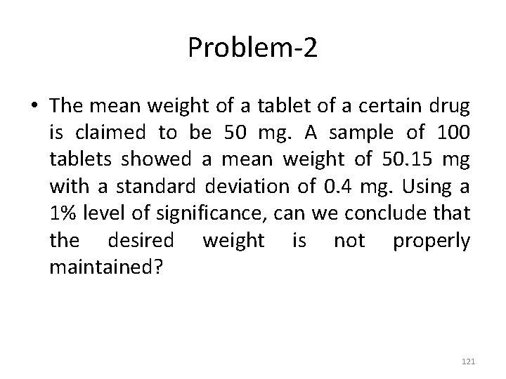
Problem-2 • The mean weight of a tablet of a certain drug is claimed to be 50 mg. A sample of 100 tablets showed a mean weight of 50. 15 mg with a standard deviation of 0. 4 mg. Using a 1% level of significance, can we conclude that the desired weight is not properly maintained? 121

Problem-2 Solution 122

Assessment problem-1 • A manufacturer supplies the rear axles for U. S Postal Service mail trucks. These axles must be able to withstand 80, 000 pounds per square inch in stress tests, but an excessively strong axle raises production costs significantly. Long experience indicates that the standard deviation of the strength of its axles is 4, 000 pounds per square inch. The manufacturer selects a sample of 100 axles from production, tests them, and finds that the mean stress capacity of the sample is 79, 600 pounds per square inch. 123

Assessment Problem-2 • It has been found from experience at the mean breaking strength of a particular brand of threads is 9. 63 N with a standard deviation of 1. 40 N. Recently a sample of 36 pieces of threads showed a mean breaking strength of 8. 93 N. Can we conclude at 5% and 1% levels of significance that the threads have become inferior? 124

Problem-3 • A company claims that the average lifetime of his product is 2000 hours. A random sample of 64 products is put on test and their lifetime in hours is recorded. The following sums are obtained from the lifetimes: Σx = 127808 and Σ(x- )2 = 9694. 6. Test the hypothesis that the manufacturer is overestimating the lifetimes of the products. Take α = 0. 01. • 125

Problem-3 Solution 126

Problem-4 • Individual filing of income tax returns prior to 30 th June had an average refund of Rs. 1200. Consider the population of last minutes filers who file their returns during the last week of June. For a random sample of 400 individuals who filed a return between 25 and 30 June, the sample mean refund was Rs. 1054 and the sample standard deviation was Rs. 1600. Using 5% level of significance, test the belief that the individuals who wait until the last week of June to file their returns to get a higher refund than early the filers. 127

Problem-4 Solution 128

Assessment Problem-3 • A package device is set to fill detergent powder packets with a mean weight of 5 kg, with standard deviation of 0. 21 kg. The weight of packets can be assumed to be normally distributed. The weight of packets is known to drift upwards over a period of time due to machine fault, which is not tolerable. A random sample of 100 packets is taken and weighted. This sample has a mean weight of 5. 03 kg. Can we conclude that the mean weight produced by the machine has increased? Use a 5% level of significance. 129

Assessment Problem-4 • The mean life span of a sample fluorescent LEDs produced by a company is found to be 1600 days with a standard deviation of 150 days. Test the hypothesis that the mean life span of fluorescent LEDs produced in general is higher than the mean life of 1570 days at α = 0. 01 level of significance. 130

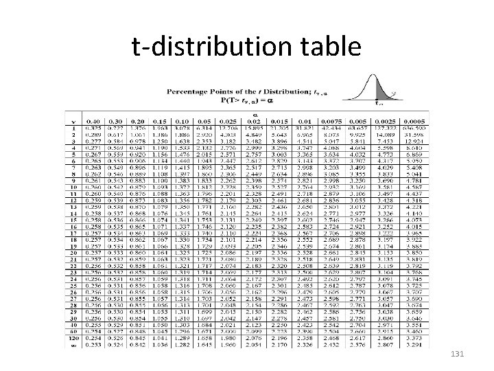
t-distribution table 131

Problem-5 • Researchers are interested in whether the mean level of enzyme B in a certain population is different from 120. They measure levels of enzyme B in a sample of 15 individuals and find that the mean, = 96 and the sample standard deviation, s = 35. 132

Problem-5 Solution 133

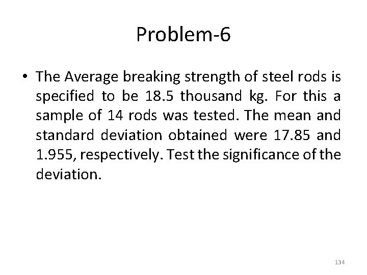
Problem-6 • The Average breaking strength of steel rods is specified to be 18. 5 thousand kg. For this a sample of 14 rods was tested. The mean and standard deviation obtained were 17. 85 and 1. 955, respectively. Test the significance of the deviation. 134

Problem-6 Solution 135

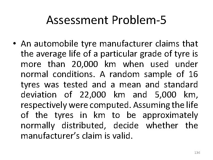
Assessment Problem-5 • An automobile tyre manufacturer claims that the average life of a particular grade of tyre is more than 20, 000 km when used under normal conditions. A random sample of 16 tyres was tested and a mean and standard deviation of 22, 000 km and 5, 000 km, respectively were computed. Assuming the life of the tyres in km to be approximately normally distributed, decide whether the manufacturer’s claim is valid. 136

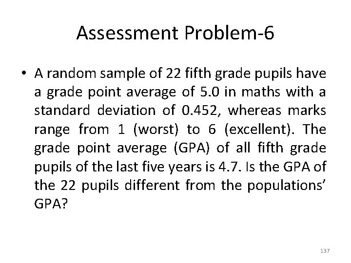
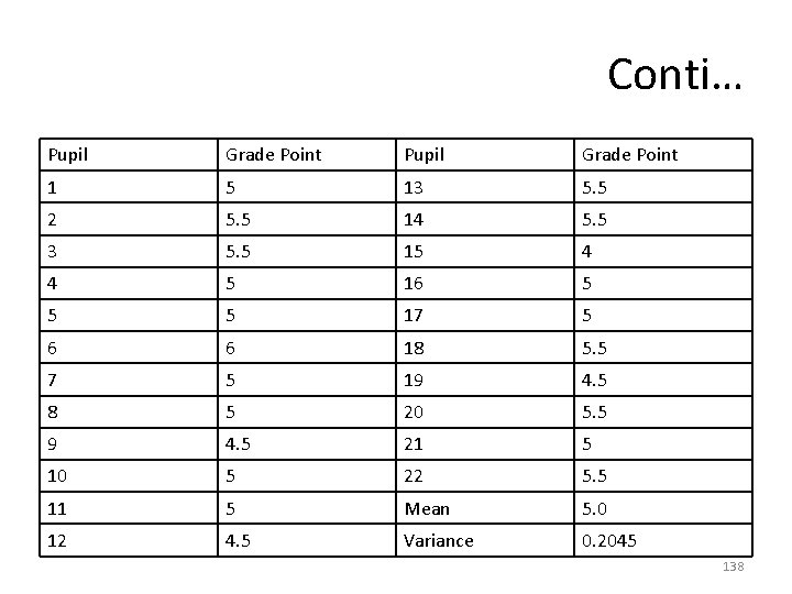
Assessment Problem-6 • A random sample of 22 fifth grade pupils have a grade point average of 5. 0 in maths with a standard deviation of 0. 452, whereas marks range from 1 (worst) to 6 (excellent). The grade point average (GPA) of all fifth grade pupils of the last five years is 4. 7. Is the GPA of the 22 pupils different from the populations’ GPA? 137

Conti… Pupil Grade Point 1 5 13 5. 5 2 5. 5 14 5. 5 3 5. 5 15 4 4 5 16 5 5 5 17 5 6 6 18 5. 5 7 5 19 4. 5 8 5 20 5. 5 9 4. 5 21 5 10 5 22 5. 5 11 5 Mean 5. 0 12 4. 5 Variance 0. 2045 138

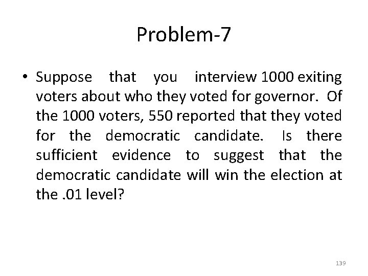
Problem-7 • Suppose that you interview 1000 exiting voters about who they voted for governor. Of the 1000 voters, 550 reported that they voted for the democratic candidate. Is there sufficient evidence to suggest that the democratic candidate will win the election at the. 01 level? 139

Problem-7 Solution 140

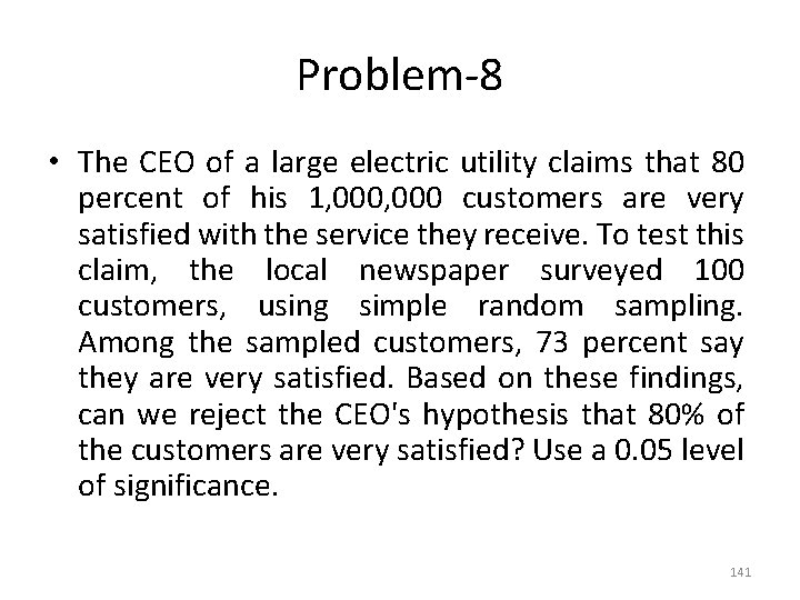
Problem-8 • The CEO of a large electric utility claims that 80 percent of his 1, 000 customers are very satisfied with the service they receive. To test this claim, the local newspaper surveyed 100 customers, using simple random sampling. Among the sampled customers, 73 percent say they are very satisfied. Based on these findings, can we reject the CEO's hypothesis that 80% of the customers are very satisfied? Use a 0. 05 level of significance. 141

Problem-8 Solution 142

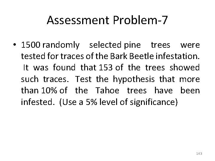
Assessment Problem-7 • 1500 randomly selected pine trees were tested for traces of the Bark Beetle infestation. It was found that 153 of the trees showed such traces. Test the hypothesis that more than 10% of the Tahoe trees have been infested. (Use a 5% level of significance) 143

Assessment Problem-8 • Suppose the CEO claims that at least 80 percent of the company's 1, 000 customers are very satisfied. Again, 100 customers are surveyed using simple random sampling. The result: 73 percent are very satisfied. Based on these results, should we accept or reject the CEO's hypothesis? Assume a significance level of 0. 05. 144

What if we have two populations? ? • So far we have discussed hypothesis testing for single parameter. • We assume that students are capable to understand the problem and decide which statistic is applicable under different conditions. • Students are also capable of designing critical region. • Final conclusion should be in the form of detailed analysis. 145

• Suppose we want to compare two population of students. • Two antibiotics are required to compare for response time. • Analysis of Performance of two machines. • Analysis of two detergents’ efficiency like whitening. • And many situations like…. 146

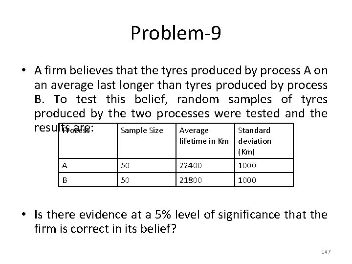
Problem-9 • A firm believes that the tyres produced by process A on an average last longer than tyres produced by process B. To test this belief, random samples of tyres produced by the two processes were tested and the results are: Process Sample Size Average Standard lifetime in Km deviation (Km) A 50 22400 1000 B 50 21800 1000 • Is there evidence at a 5% level of significance that the firm is correct in its belief? 147

Problem-9 Solution 148

Problem-10 • A random sample of size 6 from a normal population with variance 24 gave mean= 15. A sample of size 8 from a normal population with variance 80 gave mean = 13. Test the Ho= μ 1 -μ 2=0 against not equal to 0. 149

Problem-10 Solution 150

Assessment Problem • On an examination in a statistics course, the average marks of 50 boys was 72 with a population standard deviation of 8, while the average marks of 45 girls was 75. Test the hypothesis at (a) 5% and (b) 1% level of significance that the boys’ performance is inferior to that of the girls. 151

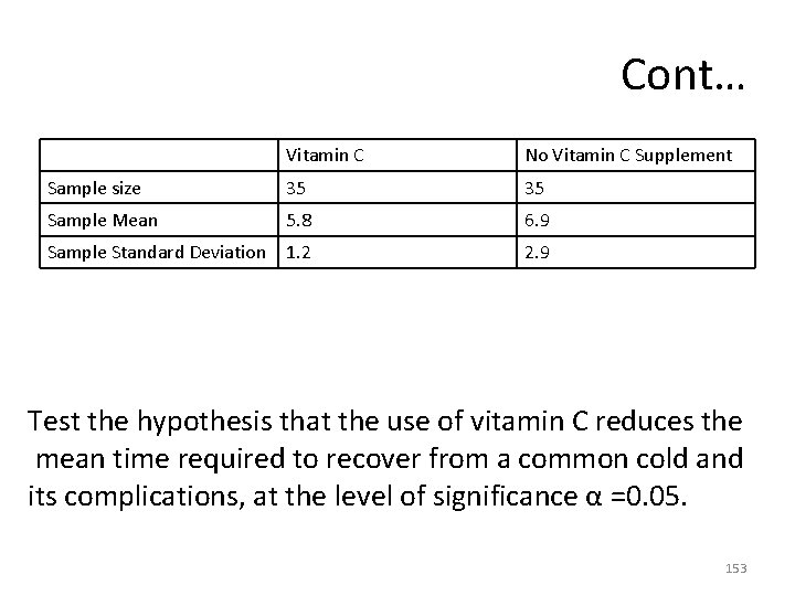
Problem-11 • An experiment was conducted to compare the mean time in days required to recover from the common cold for a person given daily dose of 4 mg of vitamin C versus those who were not given a vitamin supplement. Suppose that 35 adults were randomly selected for each treatment category and that the mean recovery times and standard devotions for the two groups were as fellows: 152

Cont… Vitamin C No Vitamin C Supplement Sample size 35 35 Sample Mean 5. 8 6. 9 Sample Standard Deviation 1. 2 2. 9 Test the hypothesis that the use of vitamin C reduces the mean time required to recover from a common cold and its complications, at the level of significance α =0. 05. 153

Problem-11 Solution 154

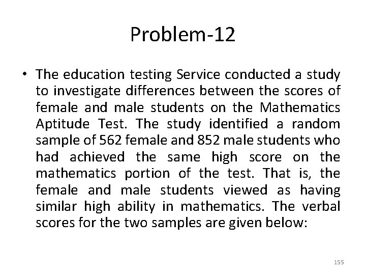
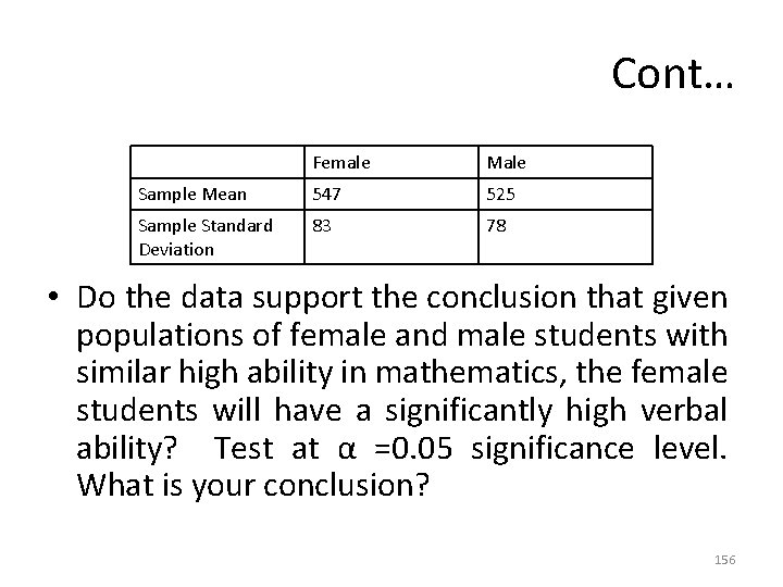
Problem-12 • The education testing Service conducted a study to investigate differences between the scores of female and male students on the Mathematics Aptitude Test. The study identified a random sample of 562 female and 852 male students who had achieved the same high score on the mathematics portion of the test. That is, the female and male students viewed as having similar high ability in mathematics. The verbal scores for the two samples are given below: 155

Cont… Female Male Sample Mean 547 525 Sample Standard Deviation 83 78 • Do the data support the conclusion that given populations of female and male students with similar high ability in mathematics, the female students will have a significantly high verbal ability? Test at α =0. 05 significance level. What is your conclusion? 156

Problem-12 Solution 157

Assessment Problem • The mean height of 50 males students of group I is 68. 2 inches with a standard deviation of 2. 5 inches, while 0 males students of group II as a mean height of 67. 5 inches with a standard deviation of 2. 8 inches. Test the hypothesis that male students of group of I are taller than male students of group II at the 0. 05 level of significance. 158

Assessment Problem • A farmer claims that the average yield of corn of variety-----variety B by at least 12 bushels per acre. ----- with a standard deviation of 6. 28 bushels per acre, while variety B yielded on average 77. 8 bushels per acre with a standard deviation of 5. 64 bushels per acre. Test the farmer’s claim using a 0. 05 level of significance. 159

Problem 13 • Suppose the Acme Drug Company develops a new drug, designed to prevent colds. The company states that the drug is equally effective for men and women. To test this claim, they choose a a simple random sample of 100 women and 200 men from a population of 100, 000 volunteers. • At the end of the study, 38% of the women caught a cold; and 51% of the men caught a cold. Based on these findings, can we reject the company's claim that the drug is equally effective for men and women? Use a 0. 05 level of significance. 160

Problem-13 Solution 161

Problem-14 • Suppose the Acme Drug Company develops a new drug, designed to prevent colds. The company states that the drug is more effective for women than for men. To test this claim, they choose a simple random sample of 100 women and 200 men from a population of 100, 000 volunteers. 162

Problem-14 Solution 163

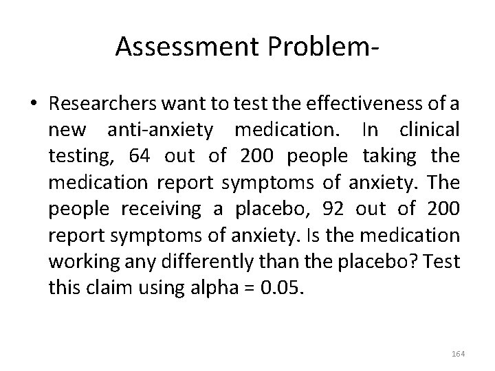
Assessment Problem • Researchers want to test the effectiveness of a new anti-anxiety medication. In clinical testing, 64 out of 200 people taking the medication report symptoms of anxiety. The people receiving a placebo, 92 out of 200 report symptoms of anxiety. Is the medication working any differently than the placebo? Test this claim using alpha = 0. 05. 164

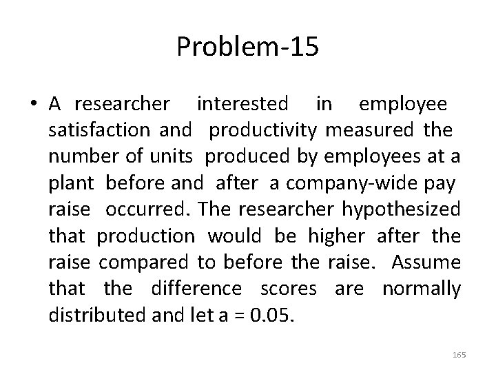
Problem-15 • A researcher interested in employee satisfaction and productivity measured the number of units produced by employees at a plant before and after a company-wide pay raise occurred. The researcher hypothesized that production would be higher after the raise compared to before the raise. Assume that the difference scores are normally distributed and let a = 0. 05. 165

Cont… Participant Before After 1 7 7 2 4 5 3 8 9 4 8 9 5 6 6 6 7 5 5 8 5 4 9 7 7 166

Problem 15 Solution 167

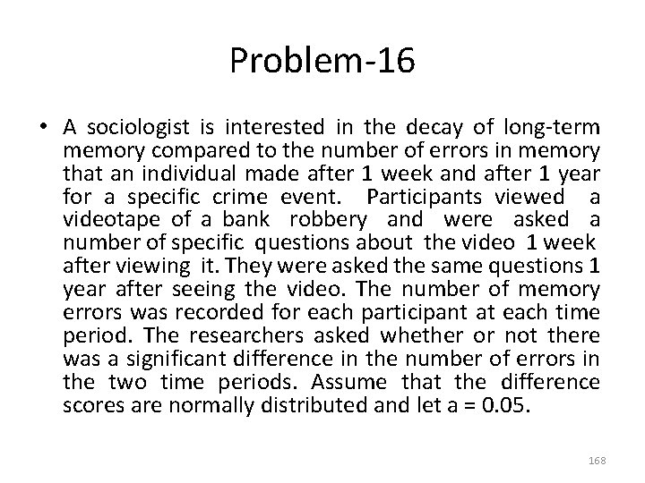
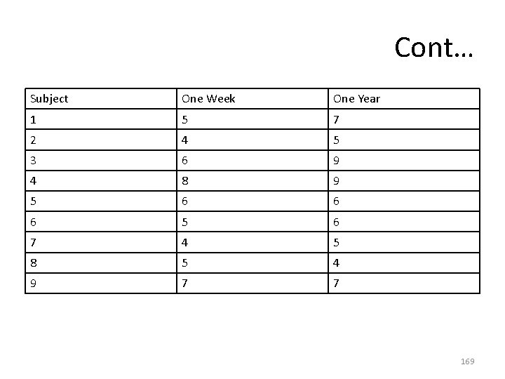
Problem-16 • A sociologist is interested in the decay of long-term memory compared to the number of errors in memory that an individual made after 1 week and after 1 year for a specific crime event. Participants viewed a videotape of a bank robbery and were asked a number of specific questions about the video 1 week after viewing it. They were asked the same questions 1 year after seeing the video. The number of memory errors was recorded for each participant at each time period. The researchers asked whether or not there was a significant difference in the number of errors in the two time periods. Assume that the difference scores are normally distributed and let a = 0. 05. 168

Cont… Subject One Week One Year 1 5 7 2 4 5 3 6 9 4 8 9 5 6 6 6 5 6 7 4 5 8 5 4 9 7 7 169

Problem-16 Solution 170

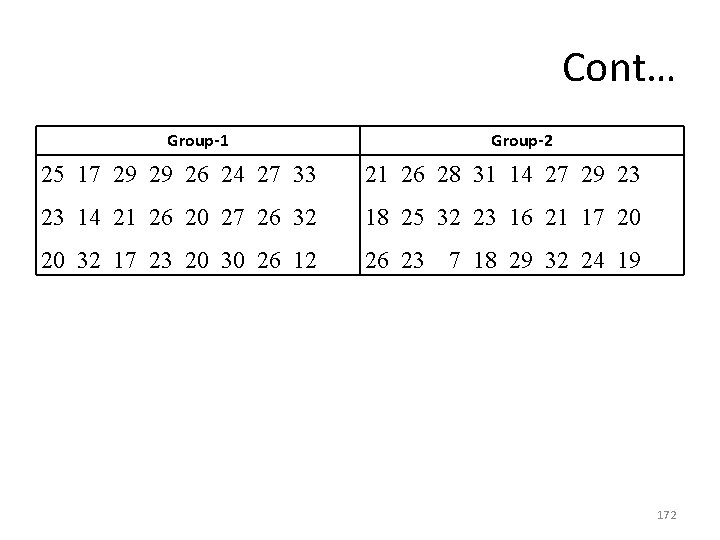
Assessment Problem • Suppose you are interested in developing a counseling technique to reduce stress within marriages. You randomly select two samples of married individuals out of ten churches in the association. You provide Group 1 with group counseling and study materials. You provide Group 2 with individual counseling and study materials. • At the conclusion of the treatment period, you measure the level of marital stress in the group members. Here are the scores: 171

Cont… Group-1 Group-2 25 17 29 29 26 24 27 33 21 26 28 31 14 27 29 23 23 14 21 26 20 27 26 32 18 25 32 23 16 21 17 20 20 32 17 23 20 30 26 12 26 23 7 18 29 32 24 19 172