Violations of Regression Assumptions Copyright c 2008 by

Violations of Regression Assumptions Copyright (c) 2008 by The Mc. Graw-Hill Companies. This spreadsheet is intended solely for educational purposes by licensed users of Learning. Stats. It may not be copied or resold for profit.

Minitab Copyright Notice Portions of MINITAB Statistical Software input and output contained in this document are printed with permission of Minitab, Inc. MINITABTM is a trademark of Minitab Inc. in the United States and other countries and is used herein with the owner's permission.

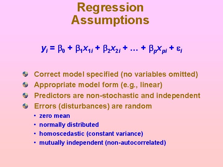
Regression Assumptions yi = b 0 + b 1 x 1 i + b 2 x 2 i + … + bpxpi + ei Correct model specified (no variables omitted) Appropriate model form (e. g. , linear) Predictors are non-stochastic and independent Errors (disturbances) are random • • zero mean normally distributed homoscedastic (constant variance) mutually independent (non-autocorrelated)

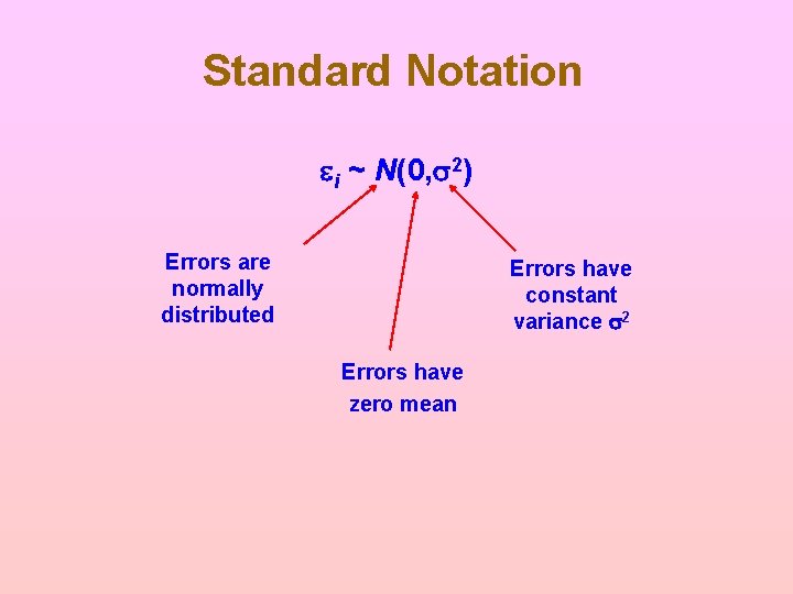
Standard Notation ei ~ N(0, s 2) Errors are normally distributed Errors have constant variance s 2 Errors have zero mean

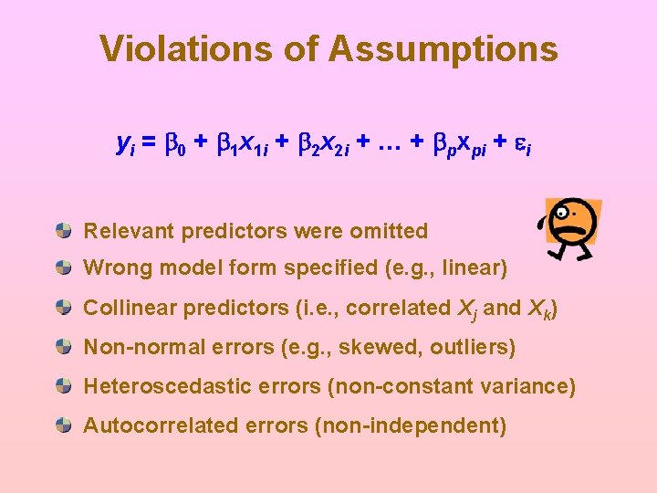
Violations of Assumptions yi = b 0 + b 1 x 1 i + b 2 x 2 i + … + bpxpi + ei Relevant predictors were omitted Wrong model form specified (e. g. , linear) Collinear predictors (i. e. , correlated Xj and Xk) Non-normal errors (e. g. , skewed, outliers) Heteroscedastic errors (non-constant variance) Autocorrelated errors (non-independent)

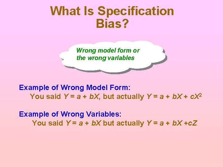
What Is Specification Bias? Wrong model form or the wrong variables Example of Wrong Model Form: You said Y = a + b. X, but actually Y = a + b. X + c. X 2 Example of Wrong Variables: You said Y = a + b. X but actually Y = a + b. X +c. Z

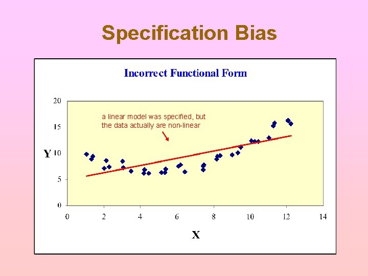
Specification Bias a linear model was specified, but the data actually are non-linear

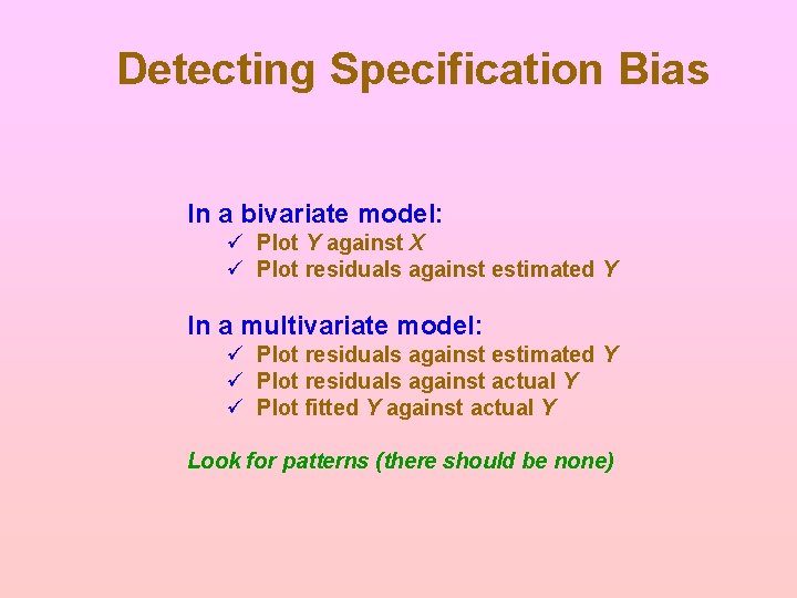
Detecting Specification Bias In a bivariate model: ü Plot Y against X ü Plot residuals against estimated Y In a multivariate model: ü Plot residuals against estimated Y ü Plot residuals against actual Y ü Plot fitted Y against actual Y Look for patterns (there should be none)

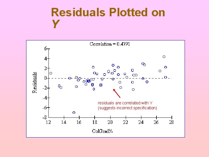
Residuals Plotted on Y residuals are correlated with Y (suggests incorrect specification)

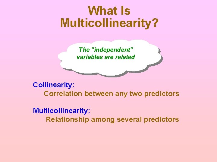
What Is Multicollinearity? The "independent" variables are related Collinearity: Correlation between any two predictors Multicollinearity: Relationship among several predictors

Effects of Multicollinearity Estimates may be unstable Standard errors may be misleading Confidence intervals generally too wide High R 2 yet t statistics insignificant

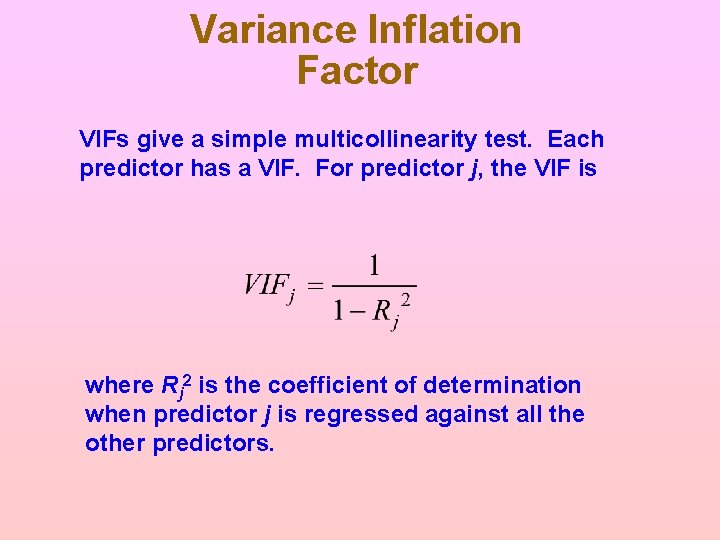
Variance Inflation Factor VIFs give a simple multicollinearity test. Each predictor has a VIF. For predictor j, the VIF is where Rj 2 is the coefficient of determination when predictor j is regressed against all the other predictors.

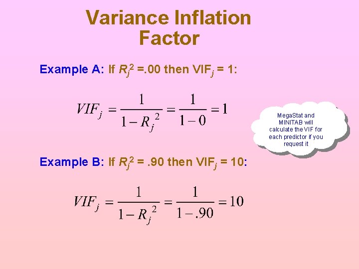
Variance Inflation Factor Example A: If Rj 2 =. 00 then VIFj = 1: Mega. Stat and MINITAB will calculate the VIF for each predictor if you request it Example B: If Rj 2 =. 90 then VIFj = 10:

Evidence of Multicollinearity Any VIF > 10 Sum of VIFs > 10 High correlation for pairs of predictors Xj and Xk Unstable estimates (i. e. , the remaining coefficients change sharply when a suspect predictor is dropped from the model)

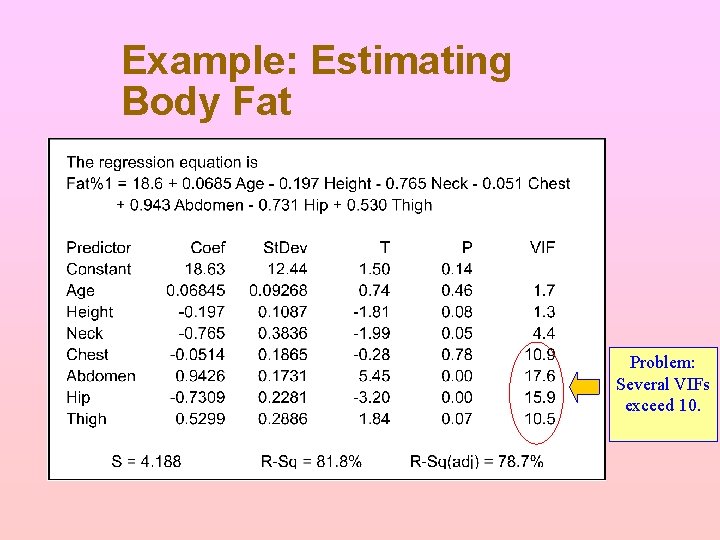
Example: Estimating Body Fat Problem: Several VIFs exceed 10.

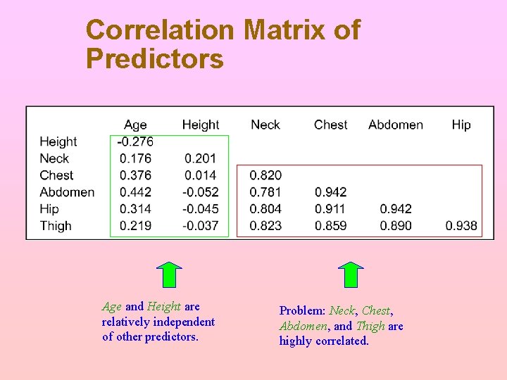
Correlation Matrix of Predictors Age and Height are relatively independent of other predictors. Problem: Neck, Chest, Abdomen, and Thigh are highly correlated.

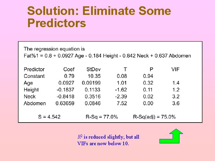
Solution: Eliminate Some Predictors R 2 is reduced slightly, but all VIFs are now below 10.

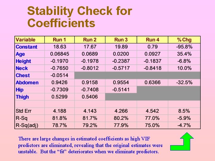
Stability Check for Coefficients There are large changes in estimated coefficients as high VIF predictors are eliminated, revealing that the original estimates were unstable. But the “fit” deteriorates when we eliminate predictors.

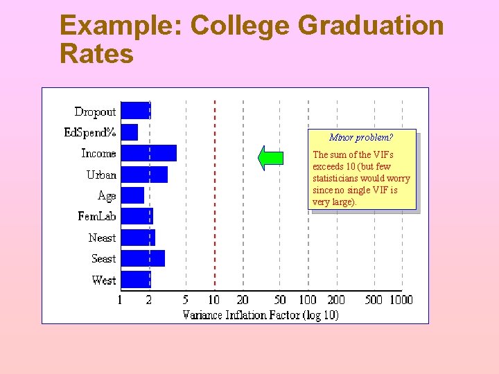
Example: College Graduation Rates Minor problem? The sum of the VIFs exceeds 10 (but few statisticians would worry since no single VIF is very large).

Remedies for Multicollinearity Drop one or more predictors But this may create specification error Transform some variables (e. g. , log X) Enlarge the sample size (if you can) Tip If they feel the model is correctly specified, statisticians tend to ignore multicollinearity unless its influence on the estimates is severe.

What Is Heteroscedasticity? Non-constant error variance Homoscedastic: Errors have the same variance for all values of the predictors (or Y) Heteroscedastic Error variance changes with the values of the predictors (or Y)

How to Detect Heteroscedasticity Excel and Mega. Stat and MINITAB will do these residual plots if you request them Plot residuals against each predictor (a bit tedious) Plot residuals against estimated Y (quick check) There are more general tests, but they are complex

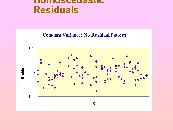
Homoscedastic Residuals

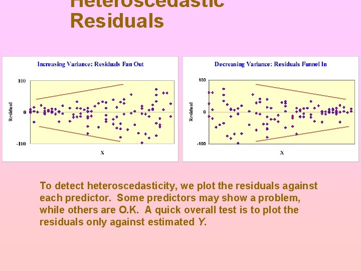
Heteroscedastic Residuals To detect heteroscedasticity, we plot the residuals against each predictor. Some predictors may show a problem, while others are O. K. A quick overall test is to plot the residuals only against estimated Y.

Effects of Heteroscedasticity Happily. . . v OLS coefficients bj are still unbiased v OLS coefficients bj are still consistent But. . . v Std errors of b's are biased (bias may be + or -) v t values and CI for b's may be unreliable v May indicate incorrect model specification

Remedies for Heteroscedasticity Avoid totals (e. g. , use per capita data) Transform some variables (e. g. , log X) Don't worry about it (may not be serious)

What Is Autocorrelation? The errors are not independent Independent errors: et does not depend on et-1 (r = 0) Autocorrelated errors: et depends on et-1 (r 0) Good News Autocorrelation is a worry in time-series models (the subscript t = 1, 2, . . . , n denotes time) but generally not in cross-sectional data.

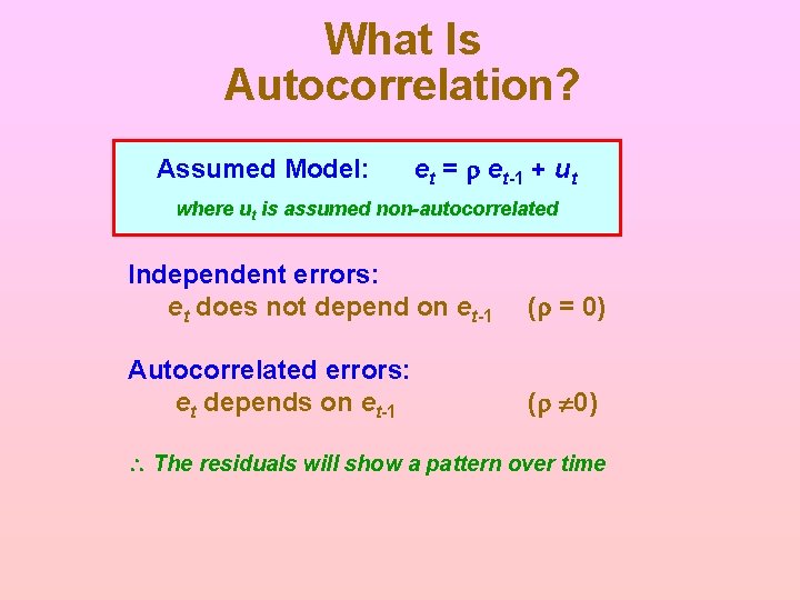
What Is Autocorrelation? Assumed Model: et = r et-1 + ut where ut is assumed non-autocorrelated Independent errors: et does not depend on et-1 (r = 0) Autocorrelated errors: et depends on et-1 (r 0) The residuals will show a pattern over time

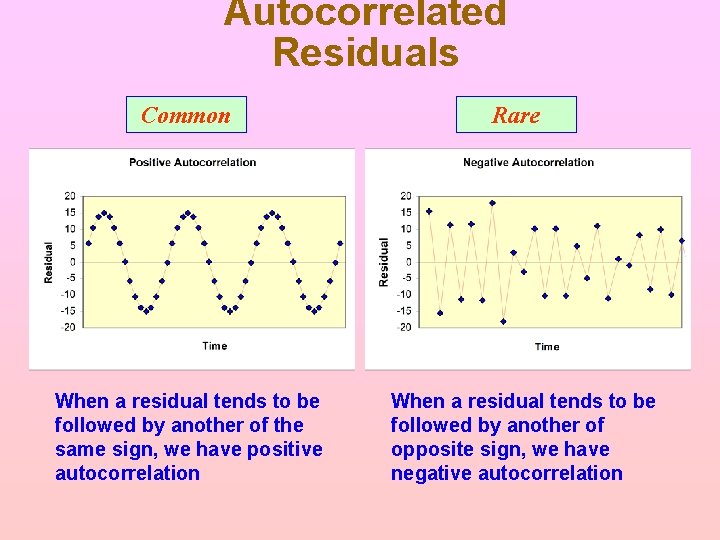
Autocorrelated Residuals Common When a residual tends to be followed by another of the same sign, we have positive autocorrelation Rare When a residual tends to be followed by another of opposite sign, we have negative autocorrelation

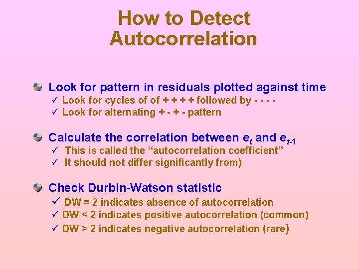
How to Detect Autocorrelation Look for pattern in residuals plotted against time ü Look for cycles of of + + followed by - - - ü Look for alternating + - pattern Calculate the correlation between et and et-1 ü This is called the “autocorrelation coefficient” ü It should not differ significantly from) Check Durbin-Watson statistic ü DW = 2 indicates absence of autocorrelation ü DW < 2 indicates positive autocorrelation (common) ü DW > 2 indicates negative autocorrelation (rare)

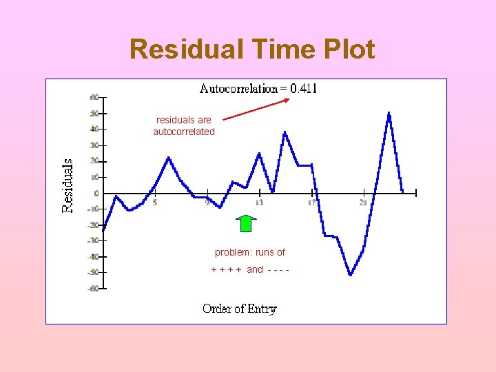
Residual Time Plot residuals are autocorrelated problem: runs of + + and - -

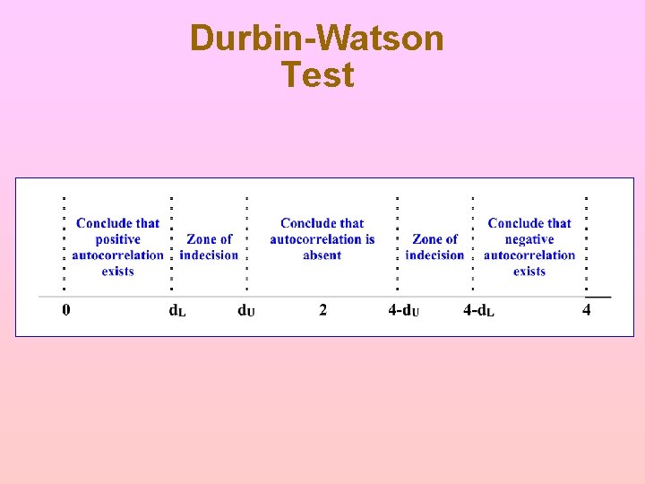
Durbin-Watson Test

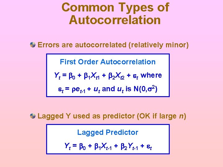
Common Types of Autocorrelation Errors are autocorrelated (relatively minor) First Order Autocorrelation Yt = b 0 + b 1 Xt 1 + b 2 Xt 2 + et where et = ret-1 + ut and ut is N(0, s 2) Lagged Y used as predictor (OK if large n) Lagged Predictor Yt = b 0 + b 1 Xt-1 + b 2 Yt-1 + et

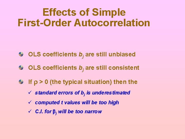
Effects of Simple First-Order Autocorrelation OLS coefficients bj are still unbiased OLS coefficients bj are still consistent If r > 0 (the typical situation) then the ü standard errors of bj is underestimated ü computed t values will be too high ü C. I. for bj will be too narrow

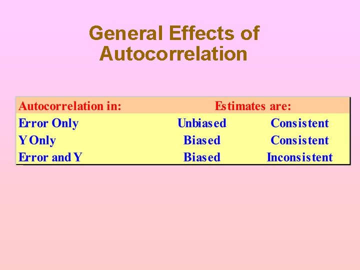
General Effects of Autocorrelation

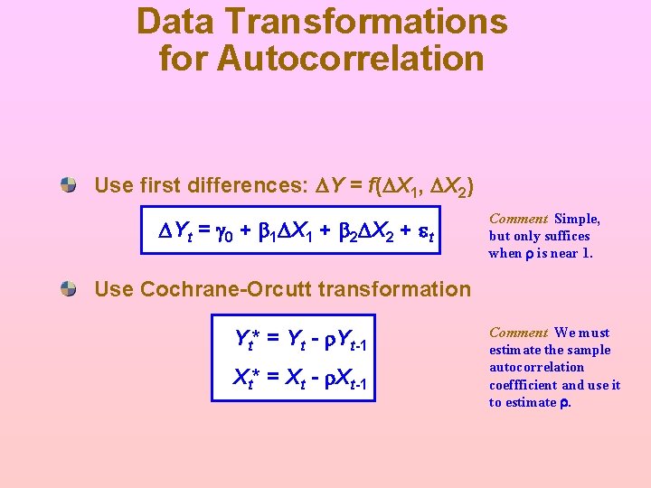
Data Transformations for Autocorrelation Use first differences: DY = f(DX 1, DX 2) DYt = g 0 + b 1 DX 1 + b 2 DX 2 + et Comment Simple, but only suffices when r is near 1. Use Cochrane-Orcutt transformation Yt* = Yt - r. Yt-1 Xt* = Xt - r. Xt-1 Comment We must estimate the sample autocorrelation coeffficient and use it to estimate r.

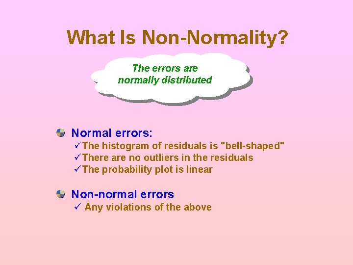
What Is Non-Normality? The errors are normally distributed Normal errors: üThe histogram of residuals is "bell-shaped" üThere are no outliers in the residuals üThe probability plot is linear Non-normal errors ü Any violations of the above

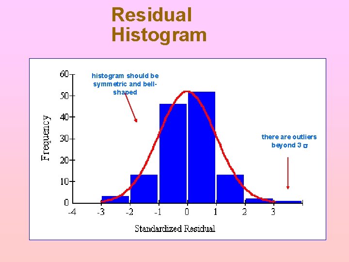
Residual Histogram histogram should be symmetric and bellshaped there are outliers beyond 3 s

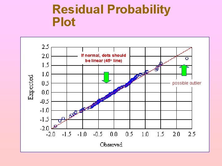
Residual Probability Plot If normal, dots should be linear (45 o line) possible outlier

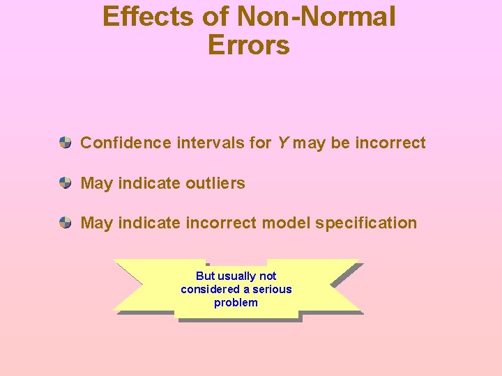
Effects of Non-Normal Errors Confidence intervals for Y may be incorrect May indicate outliers May indicate incorrect model specification But usually not considered a serious problem

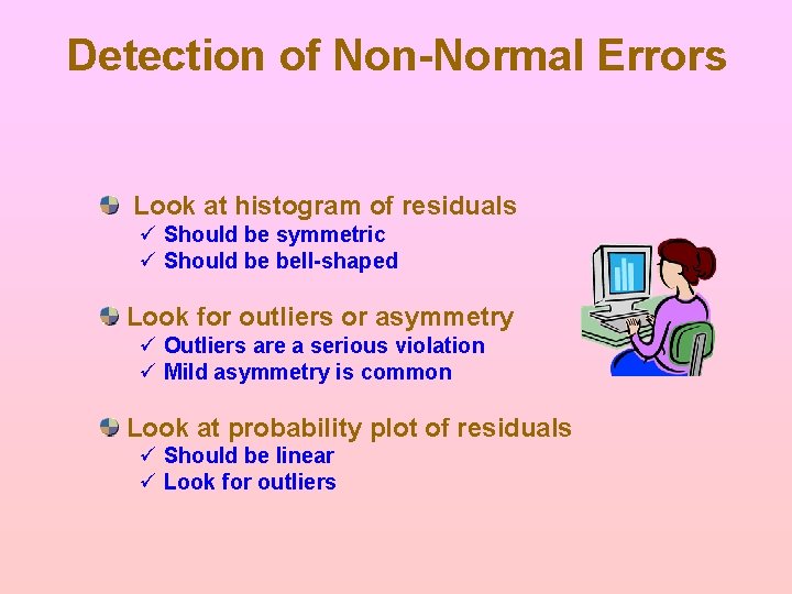
Detection of Non-Normal Errors Look at histogram of residuals ü Should be symmetric ü Should be bell-shaped Look for outliers or asymmetry ü Outliers are a serious violation ü Mild asymmetry is common Look at probability plot of residuals ü Should be linear ü Look for outliers

Remedies for Non-Normal Errors Avoid totals (e. g. , use per capita data) Transform some variables (e. g. , log X) Enlarge the sample (asymptotic normality)

Influential Observations High "leverage" of certain data points These are data points with extreme X values Sometimes called “high leverage” observations One case may strongly affect the estimates

How to Detect Influential Observations In MINITAB, look for observations denoted "X" (These are observations with unusual X values) In MINITAB, look for observations denoted "R" (These are observations with unusual residuals) Do your own tests (MINITAB does them automatically)

Rules for Finding Influential Observations Unusual X: look at hat matrix for hii > 2 p/n where ü p is the number of coefficients in the model ü n is the number of observations Unusual Y: look for large studentized deleted residuals ü Use z values as a reference if n is large ü Use t values for d. f. = n - p - 1 if n is small Unusual X and Y: use Cook’s distance measure ü Use F(p, n-p) as critical value Unusual X and Y: use MINITAB’s Dfits measure ü Rule of thumb is Dfits > 2{p/n}. 5

Remedies for Influential Observations Discard the observation only if you have logical reasons for thinking the observation is flawed Use method of least absolute deviations (but Minitab and Excel don’t calculate absolute deviations) • Call a professional statistician

Assessing Fit There are many ways The fit of a model can be assessed by ü the R 2 and R 2 adj, ü the F statistic in ANOVA table ü the standard error sy. Ix ü plot of fitted Y against actual Y

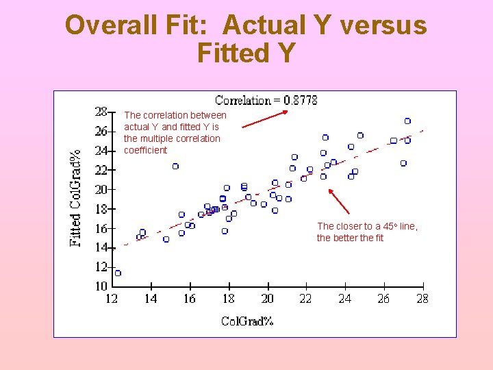
Overall Fit: Actual Y versus Fitted Y The correlation between actual Y and fitted Y is the multiple correlation coefficient The closer to a 45 o line, the better the fit

Summing It Up Computers do most of the work Regression is somewhat robust Be careful but don't panic Excelsior!