VII Factorial experiments VII A VII B VII
VII. Factorial experiments VII. A VII. B VII. C VII. D VII. E VII. F VII. G VII. H Design of factorial experiments Advantages of factorial experiments An example two-factor CRD experiment Indicator-variable models and estimation for factorial experiments Hypothesis testing using the ANOVA method for factorial experiments Treatment differences Nested factorial structures Models and hypothesis testing for three-factor experiments Statistical Modelling Chapter VII 1
Factorial experiments • Often be more than one factor of interest to the experimenter. • Definition VII. 1: Experiments that involve more than one randomized or treatment factor are called factorial experiments. • In general, the number of treatments in a factorial experiment is the product of the numbers of levels of the treatment factors. • Given the number of treatments, the experiment could be laid out as – a Completely Randomized Design, – a Randomized Complete Block Design or – a Latin Square with that number of treatments. • BIBDs or Youden Squares are not suitable. Statistical Modelling Chapter VII 2
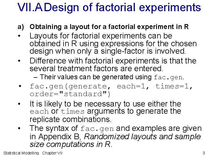
VII. ADesign of factorial experiments a) Obtaining a layout for a factorial experiment in R • • Layouts for factorial experiments can be obtained in R using expressions for the chosen design when only a single-factor is involved. Difference with factorial experiments is that the several treatment factors are entered. – Their values can be generated using fac. gen. • fac. gen(generate, each=1, times=1, order="standard") • It is likely to be necessary to use either the each or times arguments to generate the replicate combinations. • The syntax of fac. gen and examples are given in Appendix B, Randomized layouts and sample size computations in R. Statistical Modelling Chapter VII 3
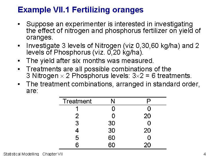
Example VII. 1 Fertilizing oranges • Suppose an experimenter is interested in investigating the effect of nitrogen and phosphorus fertilizer on yield of oranges. • Investigate 3 levels of Nitrogen (viz 0, 30, 60 kg/ha) and 2 levels of Phosphorus (viz. 0, 20 kg/ha). • The yield after six months was measured. • Treatments are all possible combinations of the 3 Nitrogen 2 Phosphorus levels: 3 2 = 6 treatments. • The treatment combinations, arranged in standard order, are: Statistical Modelling Chapter VII 4
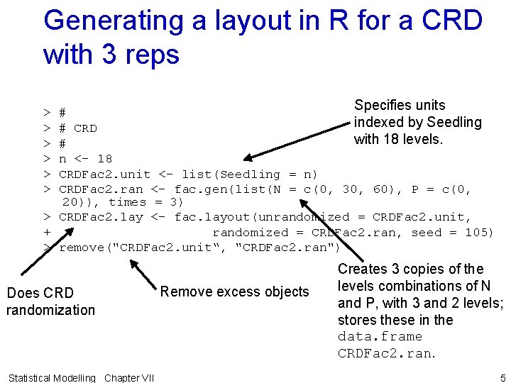
Generating a layout in R for a CRD with 3 reps Specifies units > > > # indexed by Seedling # CRD with 18 levels. # n <- 18 CRDFac 2. unit <- list(Seedling = n) CRDFac 2. ran <- fac. gen(list(N = c(0, 30, 60), P = c(0, 20)), times = 3) > CRDFac 2. lay <- fac. layout(unrandomized = CRDFac 2. unit, + randomized = CRDFac 2. ran, seed = 105) > remove("CRDFac 2. unit“, "CRDFac 2. ran") Does CRD randomization Statistical Modelling Chapter VII Remove excess objects Creates 3 copies of the levels combinations of N and P, with 3 and 2 levels; stores these in the data. frame CRDFac 2. ran. 5
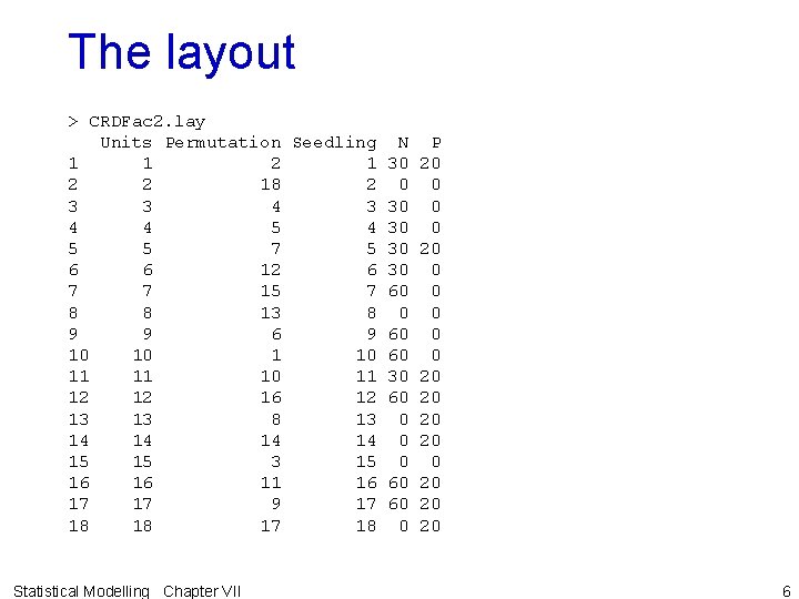
The layout > CRDFac 2. lay Units Permutation Seedling N P 1 1 2 1 30 20 2 2 18 2 0 0 3 3 4 3 30 0 4 4 5 4 30 0 5 5 7 5 30 20 6 6 12 6 30 0 7 7 15 7 60 0 8 8 13 8 0 0 9 9 60 0 10 10 1 10 60 0 11 11 10 11 30 20 12 12 16 12 60 20 13 13 8 13 0 20 14 14 0 20 15 15 3 15 0 0 16 16 11 16 60 20 17 17 9 17 60 20 18 18 17 18 0 20 Statistical Modelling Chapter VII 6
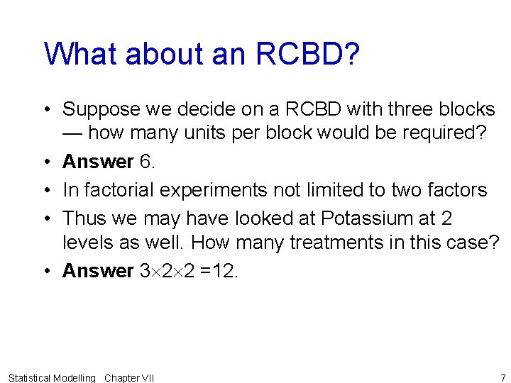
What about an RCBD? • Suppose we decide on a RCBD with three blocks — how many units per block would be required? • Answer 6. • In factorial experiments not limited to two factors • Thus we may have looked at Potassium at 2 levels as well. How many treatments in this case? • Answer 3 2 2 =12. Statistical Modelling Chapter VII 7
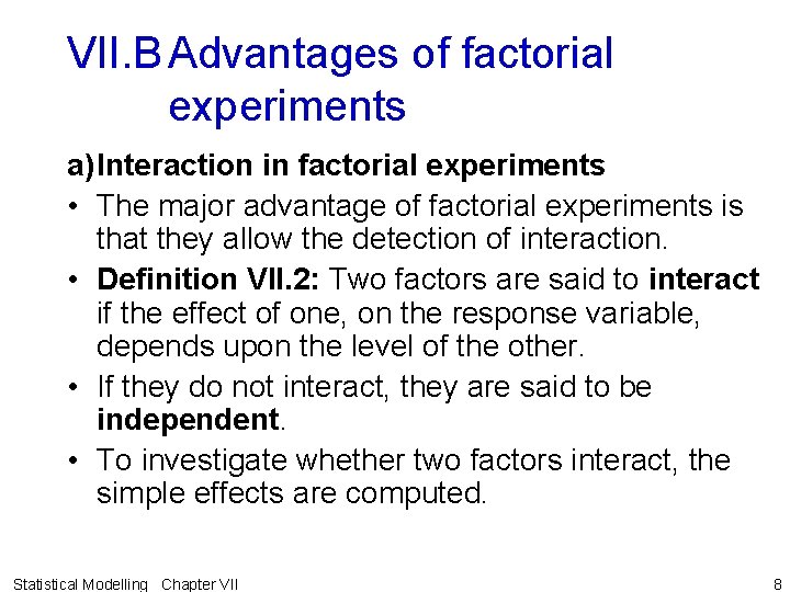
VII. B Advantages of factorial experiments a)Interaction in factorial experiments • The major advantage of factorial experiments is that they allow the detection of interaction. • Definition VII. 2: Two factors are said to interact if the effect of one, on the response variable, depends upon the level of the other. • If they do not interact, they are said to be independent. • To investigate whether two factors interact, the simple effects are computed. Statistical Modelling Chapter VII 8
Effects • Definition VII. 3: A simple effect, for the means computed for each combination of at least two factors, is the difference between two of these means having different levels of one of the factors but the same levels for all other factors. • We talk of the simple effects of a factor for the levels of the other factors. • If there is an interaction, compute an interaction effect from the simple effects to measure the size of the interaction • Definition VII. 4: An interaction effect is half the difference of two simple effects for two different levels of just one factor (or is half the difference of two interaction effects). • If there is not an interaction, can separately compute the main effects to see how each factor affects the response. • Definition VII. 5: A main effect of a factor is the difference between two means with different levels of that factor, each mean having been formed from all observations having the same level of the factor. 9 Statistical Modelling Chapter VII
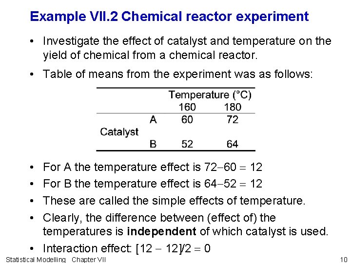
Example VII. 2 Chemical reactor experiment • Investigate the effect of catalyst and temperature on the yield of chemical from a chemical reactor. • Table of means from the experiment was as follows: • • For A the temperature effect is 72 -60 = 12 For B the temperature effect is 64 -52 = 12 These are called the simple effects of temperature. Clearly, the difference between (effect of) the temperatures is independent of which catalyst is used. • Interaction effect: [12 - 12]/2 = 0 Statistical Modelling Chapter VII 10
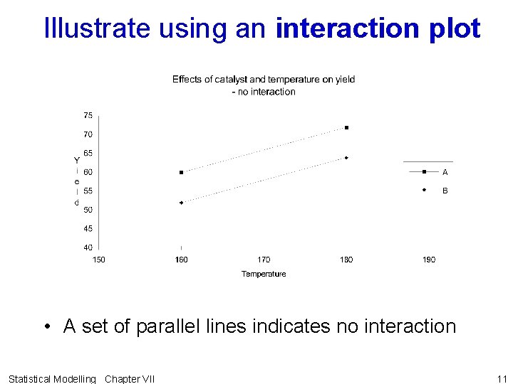
Illustrate using an interaction plot • A set of parallel lines indicates no interaction Statistical Modelling Chapter VII 11
Interaction & independence are symmetrical in factors • Thus, – the simple catalyst effect at 160°C is 52 -60 = -8 – the simple catalyst effect at 180°C is 64 -72 = -8 • Thus the difference between (effect of) the catalysts is independent of which temperature is used. • Interaction effect is still 0 and factors are additive. Statistical Modelling Chapter VII 12
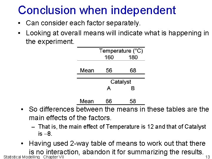
Conclusion when independent • Can consider each factor separately. • Looking at overall means will indicate what is happening in the experiment. • So differences between the means in these tables are the main effects of the factors. – That is, the main effect of Temperature is 12 and that of Catalyst is -8. • Having used 2 -way table of means to work out that there is no interaction, abandon it for summarizing the results. Statistical Modelling Chapter VII 13
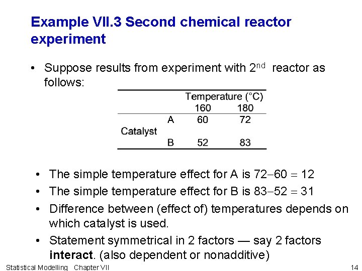
Example VII. 3 Second chemical reactor experiment • Suppose results from experiment with 2 nd reactor as follows: • The simple temperature effect for A is 72 -60 = 12 • The simple temperature effect for B is 83 -52 = 31 • Difference between (effect of) temperatures depends on which catalyst is used. • Statement symmetrical in 2 factors — say 2 factors interact. (also dependent or nonadditive) Statistical Modelling Chapter VII 14
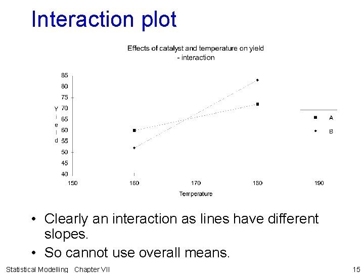
Interaction plot • Clearly an interaction as lines have different slopes. • So cannot use overall means. Statistical Modelling Chapter VII 15
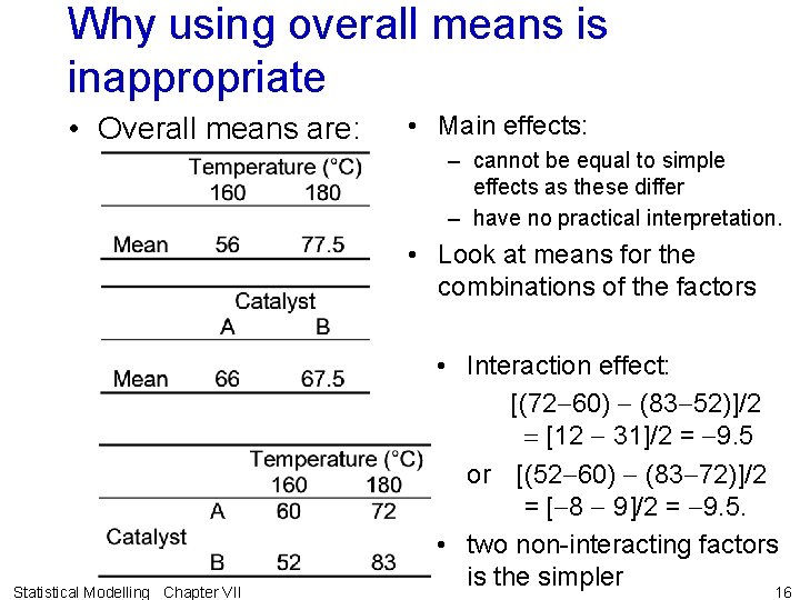
Why using overall means is inappropriate • Overall means are: • Main effects: – cannot be equal to simple effects as these differ – have no practical interpretation. • Look at means for the combinations of the factors Statistical Modelling Chapter VII • Interaction effect: [(72 -60) - (83 -52)]/2 = [12 - 31]/2 = -9. 5 or [(52 -60) - (83 -72)]/2 = [-8 - 9]/2 = -9. 5. • two non-interacting factors is the simpler 16
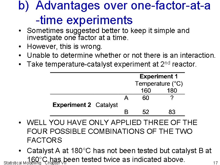
b) Advantages over one-factor-at-a -time experiments • Sometimes suggested better to keep it simple and investigate one factor at a time. • However, this is wrong. • Unable to determine whether or not there is an interaction. • Take temperature-catalyst experiment at 2 nd reactor. • WELL YOU HAVE ONLY APPLIED THREE OF THE FOUR POSSIBLE COMBINATIONS OF THE TWO FACTORS • Catalyst A at 180°C has not been tested but catalyst B at 160°C has been tested twice as indicated above. 17 Statistical Modelling Chapter VII
Limitation of inability to detect interaction • The results of the experiments would indicate that: – temperature increases yield by 31 gms – the catalysts differ by 8 gms in yield. • If we presume the factors act additively, predict the yield for catalyst A at 160°C to be: – 60+31 = 83 + 8 = 91. • This is quite clearly erroneous. • Need the factorial experiment to determine if there is an interaction. Statistical Modelling Chapter VII 18
Same resources but more info • Exactly the same total amount of resources are involved in the two alternative strategies, assuming the number of replicates is the same in all the experiments. • In addition, if the factors are additive then the main effects are estimated with greater precision in factorial experiments. • In the one-factor-at-a time experiments – the effect of a particular factor is estimated as the difference between two means each based on r observations. • In the factorial experiment – the main effects of the factors are the difference between two means based on 2 r observations – which represents a sqrt(2) increase in precision. • The improvement in precision will be greater for more factors and more levels Statistical Modelling Chapter VII 19
Summary of advantages of factorial experiments if the factors interact, factorial experiments allow this to be detected and estimates of the interaction effect can be obtained, and if the factors are independent, factorial experiments result in the estimation of the main effects with greater precision. Statistical Modelling Chapter VII 20
VII. C An example two-factor CRD experiment • Modification of ANOVA: instead of a single source for treatments, will have a source for each factor and one for each possible combinations of factors. Statistical Modelling Chapter VII 21
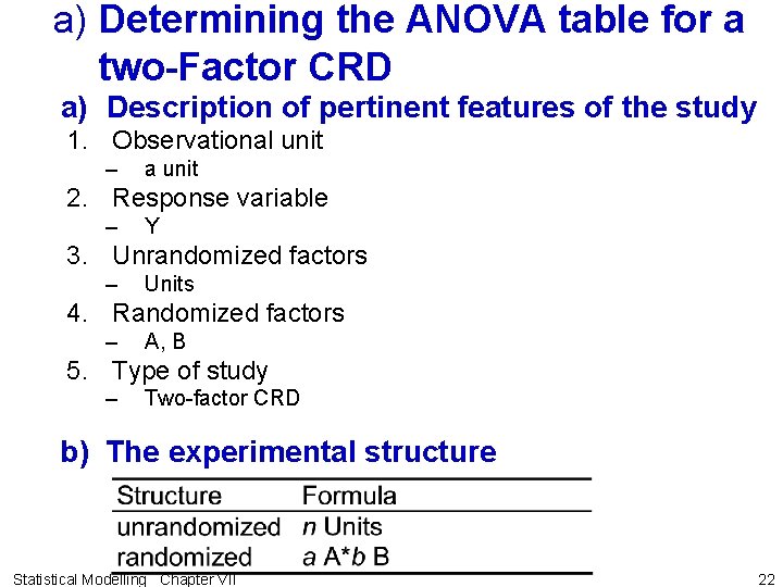
a) Determining the ANOVA table for a two-Factor CRD a) Description of pertinent features of the study 1. Observational unit – a unit 2. Response variable – Y 3. Unrandomized factors – Units 4. Randomized factors – A, B 5. Type of study – Two-factor CRD b) The experimental structure Statistical Modelling Chapter VII 22

c) Sources derived from the structure formulae • Units • A*B = Units = A + B + A#B d) Degrees of freedom and sums of squares • Hasse diagrams for this study with – degrees of freedom – M and Q matrices Statistical Modelling Chapter VII 23
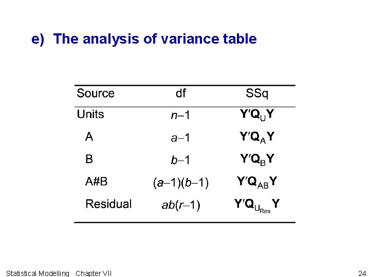
e) The analysis of variance table Statistical Modelling Chapter VII 24
f) Maximal expectation and variation models • Assume the randomized factors are fixed and that the unrandomized factor is a random factor. • Then the potential expectation terms are A, B and A B. • The variation term is: Units. • The maximal expectation model is – y = E[Y] = A B • and the variation model is – var[Y] = Units Statistical Modelling Chapter VII 25

g) The expected mean squares • The Hasse diagrams, with contributions to expected mean squares, for this study are: Statistical Modelling Chapter VII 26
![ANOVA table with E[MSq] Statistical Modelling Chapter VII 27 ANOVA table with E[MSq] Statistical Modelling Chapter VII 27](http://slidetodoc.com/presentation_image_h/004fbee1f5ba79cd59e79fbef1f3d024/image-27.jpg)
ANOVA table with E[MSq] Statistical Modelling Chapter VII 27
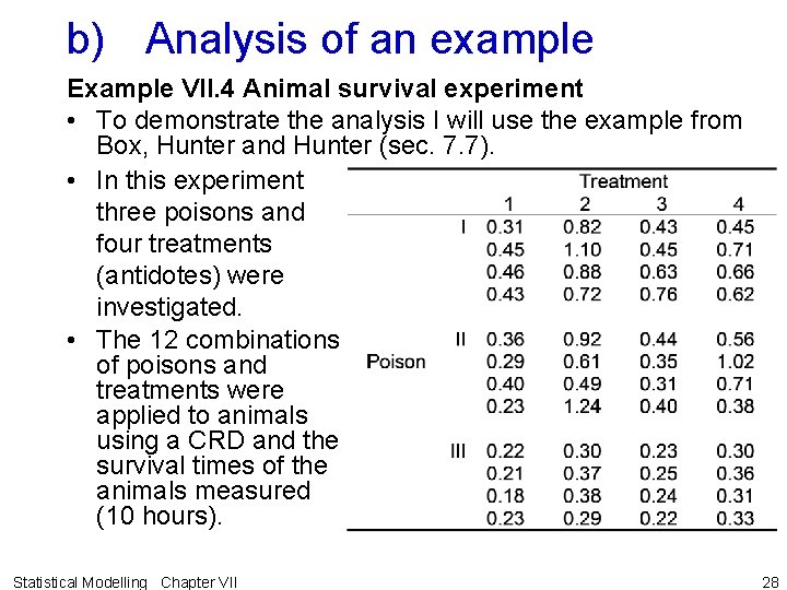
b) Analysis of an example Example VII. 4 Animal survival experiment • To demonstrate the analysis I will use the example from Box, Hunter and Hunter (sec. 7. 7). • In this experiment three poisons and four treatments (antidotes) were investigated. • The 12 combinations of poisons and treatments were applied to animals using a CRD and the survival times of the animals measured (10 hours). Statistical Modelling Chapter VII 28
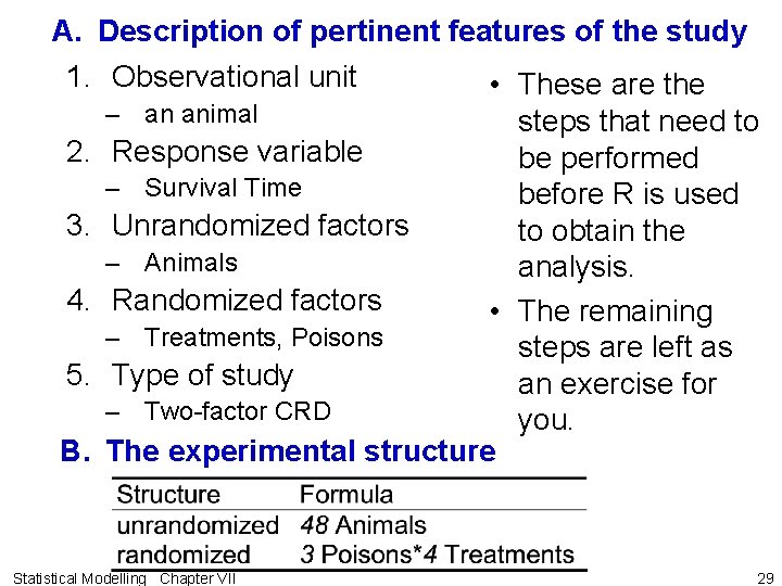
A. Description of pertinent features of the study 1. Observational unit • These are the – an animal steps that need to 2. Response variable be performed – Survival Time before R is used 3. Unrandomized factors to obtain the – Animals analysis. 4. Randomized factors • The remaining – Treatments, Poisons steps are left as 5. Type of study an exercise for – Two-factor CRD you. B. The experimental structure Statistical Modelling Chapter VII 29
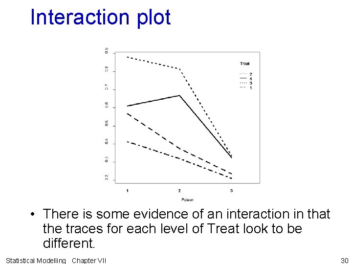
Interaction plot • There is some evidence of an interaction in that the traces for each level of Treat look to be different. Statistical Modelling Chapter VII 30
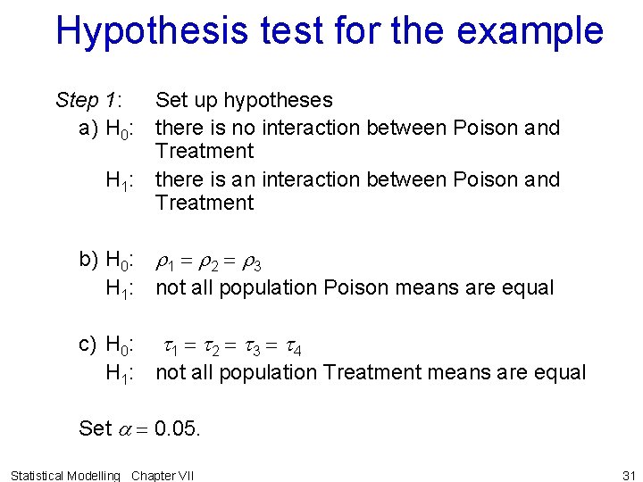
Hypothesis test for the example Step 1: Set up hypotheses a) H 0: there is no interaction between Poison and Treatment H 1: there is an interaction between Poison and Treatment b) H 0: r 1 = r 2 = r 3 H 1: not all population Poison means are equal c) H 0: t 1 = t 2 = t 3 = t 4 H 1: not all population Treatment means are equal Set a = 0. 05. Statistical Modelling Chapter VII 31
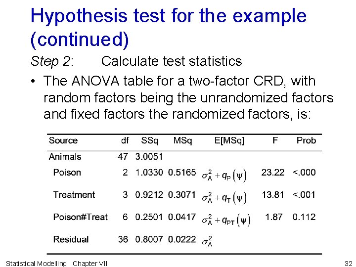
Hypothesis test for the example (continued) Step 2: Calculate test statistics • The ANOVA table for a two-factor CRD, with random factors being the unrandomized factors and fixed factors the randomized factors, is: Statistical Modelling Chapter VII 32
Hypothesis test for the example (continued) Step 3: Decide between hypotheses Interaction of Poison and Treatment is not significant, so there is no interaction. Both main effects are highly significant, so both factors affect the response. More about models soon. • Also, it remains to perform the usual diagnostic checking. Statistical Modelling Chapter VII 33
VII. DIndicator-variable models and estimation for factorial experiments • The models for the factorial experiments will depend on the design used in assigning the treatments — that is, CRD, RCBD or LS. • The design will determine the unrandomized factors and the terms to be included involving those factors. • They will also depend on the number of randomized factors. • Let the total number of observations be n and the factors be A and B with a and b levels, respectively. • Suppose that the combinations of A and B are each replicated r times — that is, n = a b r. Statistical Modelling Chapter VII 34
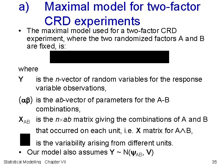
a) Maximal model for two-factor CRD experiments • The maximal model used for a two-factor CRD experiment, where the two randomized factors A and B are fixed, is: where Y is the n-vector of random variables for the response variable observations, (ab) is the ab-vector of parameters for the A-B combinations, XAB is the n ab matrix giving the combinations of A and B that occurred on each unit, i. e. X matrix for A B, is the variability arising from different units. • Our model also assumes Y ~ N(y. AB, V) Statistical Modelling Chapter VII 35
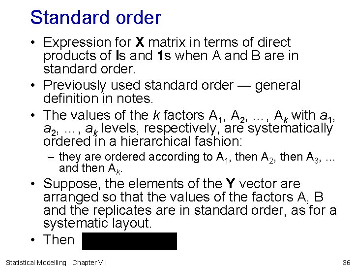
Standard order • Expression for X matrix in terms of direct products of Is and 1 s when A and B are in standard order. • Previously used standard order — general definition in notes. • The values of the k factors A 1, A 2, …, Ak with a 1, a 2, …, ak levels, respectively, are systematically ordered in a hierarchical fashion: – they are ordered according to A 1, then A 2, then A 3, … and then Ak. • Suppose, the elements of the Y vector are arranged so that the values of the factors A, B and the replicates are in standard order, as for a systematic layout. • Then Statistical Modelling Chapter VII 36
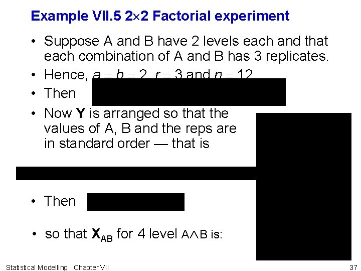
Example VII. 5 2 2 Factorial experiment • Suppose A and B have 2 levels each and that each combination of A and B has 3 replicates. • Hence, a = b = 2, r = 3 and n = 12. • Then • Now Y is arranged so that the values of A, B and the reps are in standard order — that is • Then • so that XAB for 4 level A B is: Statistical Modelling Chapter VII 37
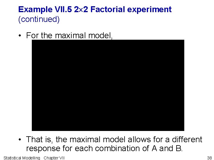
Example VII. 5 2 2 Factorial experiment (continued) • For the maximal model, • That is, the maximal model allows for a different response for each combination of A and B. Statistical Modelling Chapter VII 38
b) Alternative expectation models — marginality-compliant models Rule VII. 1: The set of expectation models corresponds to the set of all possible combinations of potential expectation terms, subject to restriction that terms marginal to another expectation term are excluded from the model; • it includes the minimal model that consists of a single term for the grand mean. • For marginality of terms refer to Hasse diagrams and can be deduced using definition VI. 9. • This definition states that one generalized factor is marginal to another if – the factors in the marginal generalized factor are a subset of those in the other and – this will occur irrespective of the replication of the levels of the generalized factors. Statistical Modelling Chapter VII 39
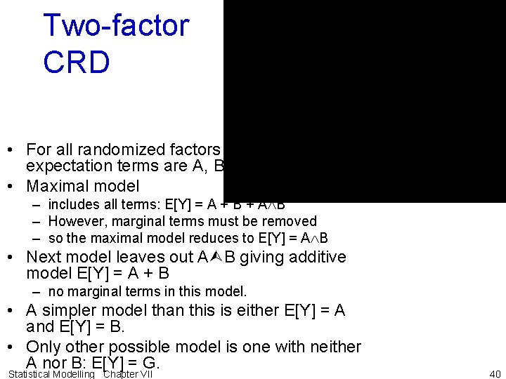
Two-factor CRD • For all randomized factors fixed, the potential expectation terms are A, B and A B. • Maximal model – includes all terms: E[Y] = A + B + A B – However, marginal terms must be removed – so the maximal model reduces to E[Y] = A B • Next model leaves out A B giving additive model E[Y] = A + B – no marginal terms in this model. • A simpler model than this is either E[Y] = A and E[Y] = B. • Only other possible model is one with neither A nor B: E[Y] = G. Statistical Modelling Chapter VII 40
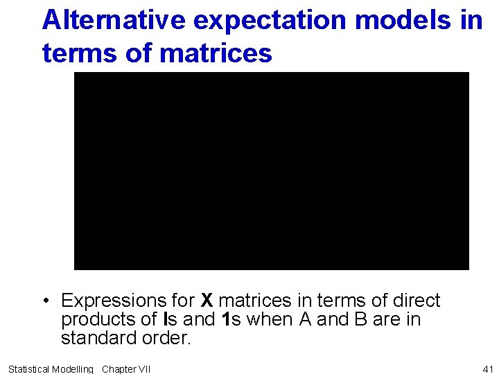
Alternative expectation models in terms of matrices • Expressions for X matrices in terms of direct products of Is and 1 s when A and B are in standard order. Statistical Modelling Chapter VII 41
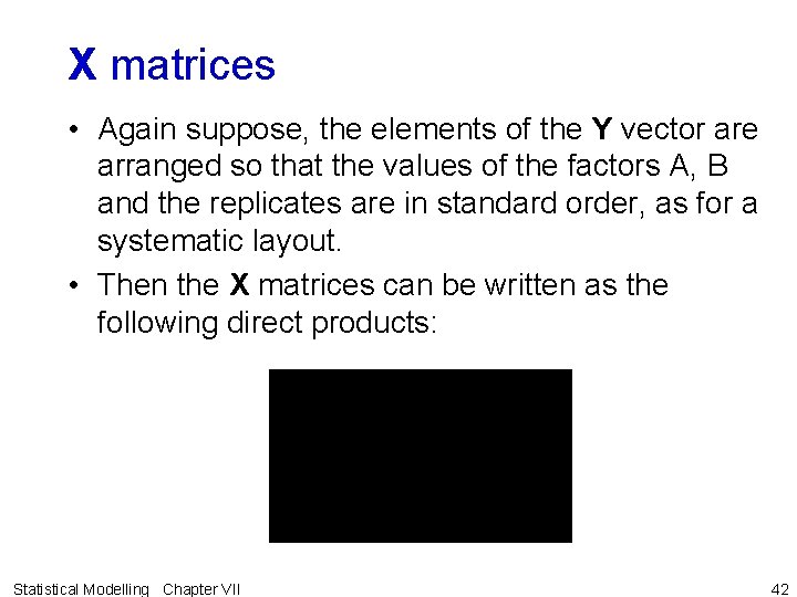
X matrices • Again suppose, the elements of the Y vector are arranged so that the values of the factors A, B and the replicates are in standard order, as for a systematic layout. • Then the X matrices can be written as the following direct products: Statistical Modelling Chapter VII 42
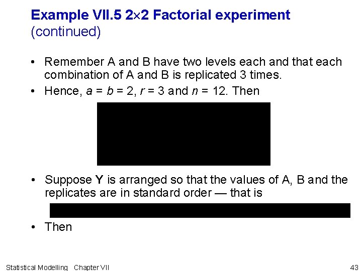
Example VII. 5 2 2 Factorial experiment (continued) • Remember A and B have two levels each and that each combination of A and B is replicated 3 times. • Hence, a = b = 2, r = 3 and n = 12. Then • Suppose Y is arranged so that the values of A, B and the replicates are in standard order — that is • Then Statistical Modelling Chapter VII 43
Example VII. 5 2 2 Factorial experiment (continued) Notice, irrespective of the replication of the levels of A B , • XG can be written as a linear combination of the columns of each of the other three • XA and XB can be written as linear combinations of the columns of XAB. Statistical Modelling Chapter VII 44
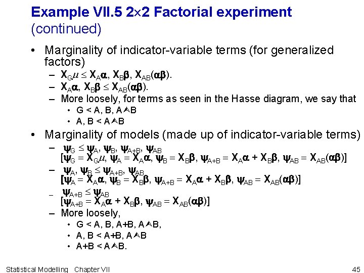
Example VII. 5 2 2 Factorial experiment (continued) • Marginality of indicator-variable terms (for generalized factors) – XGm XAa, XBb, XAB(ab). – XAa, XBb XAB(ab). – More loosely, for terms as seen in the Hasse diagram, we say that • G < A, B, A B • A, B < A B • Marginality of models (made up of indicator-variable terms) – y. G y. A, y. B, y. A+B, y. AB [y. G = XGm, y. A = XAa, y. B = XBb, y. A+B = XAa + XBb, y. AB = XAB(ab)] – y. A, y. B y. A+B, y. AB [y. A = XAa, y. B = XBb, y. A+B = XAa + XBb, y. AB = XAB(ab)] – y. A+B y. AB [y. A+B = XAa + XBb, y. AB = XAB(ab)] – More loosely, • G < A, B, A+B, A B, • A, B < A+B, A B • A+B < A B. Statistical Modelling Chapter VII 45
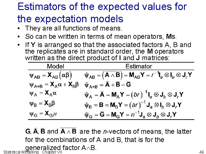
Estimators of the expected values for the expectation models • They are all functions of means. • So can be written in terms of mean operators, Ms. • If Y is arranged so that the associated factors A, B and the replicates are in standard order, the M operators written as the direct product of I and J matrices: are the n-vectors of means, the latter for the combinations of A and B, that is for the generalized factor A B. Statistical Modelling Chapter VII 46
Example VII. 5 2 2 Factorial experiment (continued) • The mean vectors, produced by an MY, are as follows: Statistical Modelling Chapter VII 47
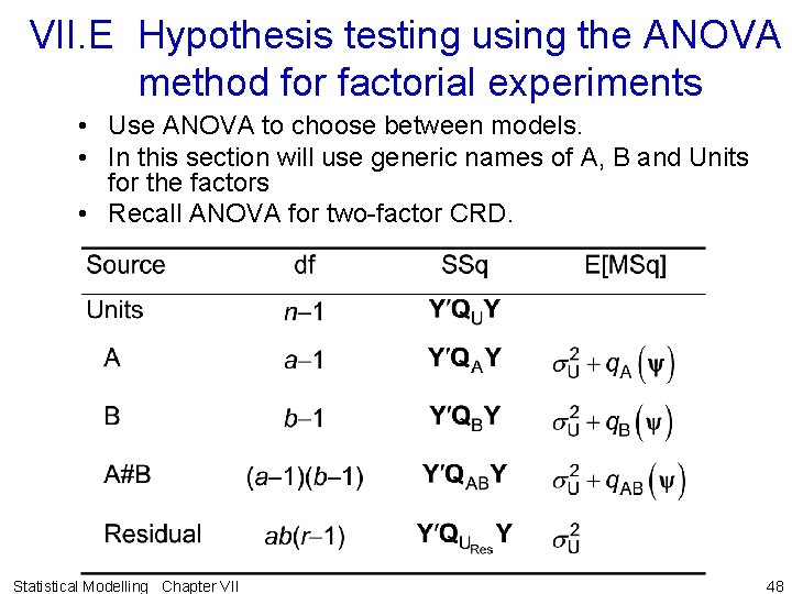
VII. E Hypothesis testing using the ANOVA method for factorial experiments • Use ANOVA to choose between models. • In this section will use generic names of A, B and Units for the factors • Recall ANOVA for two-factor CRD. Statistical Modelling Chapter VII 48
a) Sums of squares for the analysis of variance • Require estimators of the following SSqs for a two -factor CRD ANOVA: – Total or Units; A; B; A#B and Residual. • Use Hasse diagram. Statistical Modelling Chapter VII 49
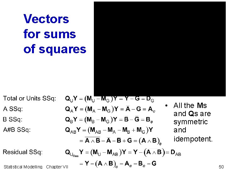
Vectors for sums of squares • All the Ms and Qs are symmetric and idempotent. Statistical Modelling Chapter VII 50
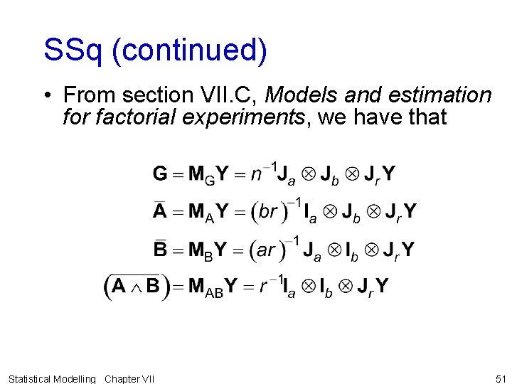
SSq (continued) • From section VII. C, Models and estimation for factorial experiments, we have that Statistical Modelling Chapter VII 51
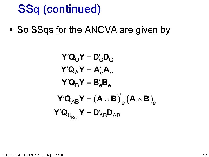
SSq (continued) • So SSqs for the ANOVA are given by Statistical Modelling Chapter VII 52
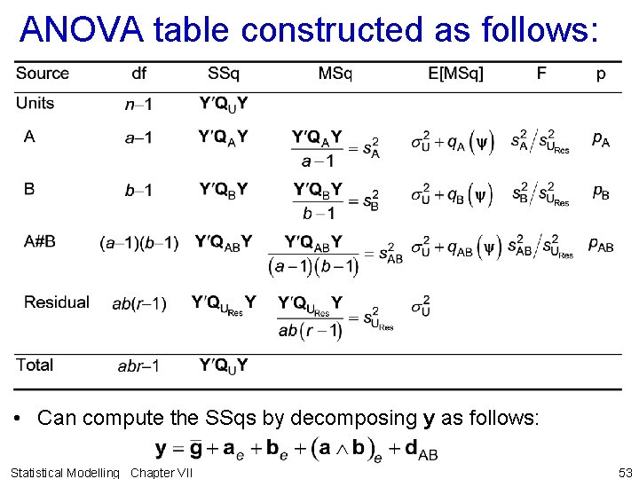
ANOVA table constructed as follows: • Can compute the SSqs by decomposing y as follows: Statistical Modelling Chapter VII 53
![d) Expected mean squares • The E[MSq]s involve three quadratic functions of the expectation d) Expected mean squares • The E[MSq]s involve three quadratic functions of the expectation](http://slidetodoc.com/presentation_image_h/004fbee1f5ba79cd59e79fbef1f3d024/image-54.jpg)
d) Expected mean squares • The E[MSq]s involve three quadratic functions of the expectation vector: • That is, numerators are SSqs of – QAy = (MA-MG)y, – QBy = (MB-MG)y and – QABy = (MAB-MA-MB+MG)y, where y is one of the models – y. G = XGm – y. A = XAa – y. B = XBb – y. A+B = XAa + XBb – y. AB = XAB(ab) Statistical Modelling Chapter VII • Require expressions for the quadratic functions under each of these models. 54
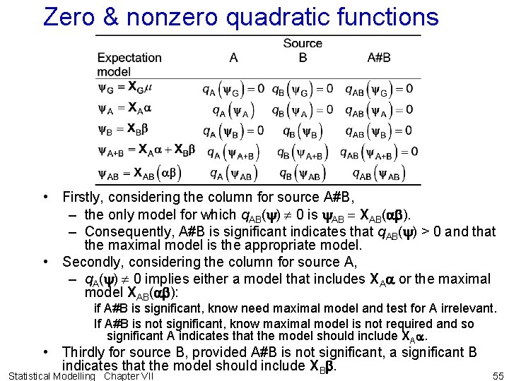
Zero & nonzero quadratic functions • Firstly, considering the column for source A#B, – the only model for which q. AB(y) 0 is y. AB = XAB(ab). – Consequently, A#B is significant indicates that q. AB(y) > 0 and that the maximal model is the appropriate model. • Secondly, considering the column for source A, – q. A(y) 0 implies either a model that includes XAa or the maximal model XAB(ab): if A#B is significant, know need maximal model and test for A irrelevant. If A#B is not significant, know maximal model is not required and so significant A indicates that the model should include XAa. • Thirdly for source B, provided A#B is not significant, a significant B indicates that the model should include XBb. Statistical Modelling Chapter VII 55

Choosing an expectation model for a two-factor CRD Statistical Modelling Chapter VII 56
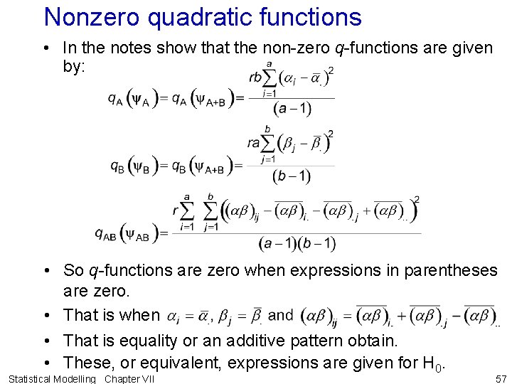
Nonzero quadratic functions • In the notes show that the non-zero q-functions are given by: • So q-functions are zero when expressions in parentheses are zero. • That is when • That is equality or an additive pattern obtain. • These, or equivalent, expressions are given for H 0. Statistical Modelling Chapter VII 57
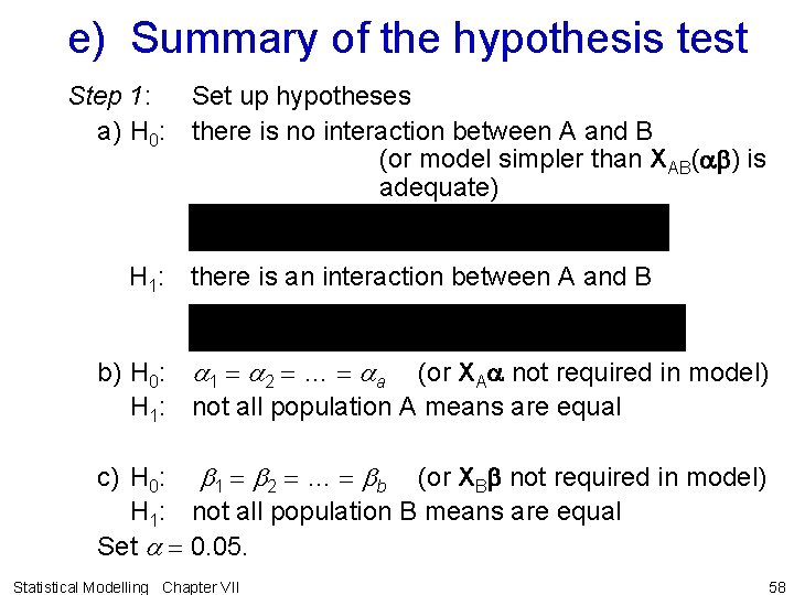
e) Summary of the hypothesis test Step 1: Set up hypotheses a) H 0: there is no interaction between A and B (or model simpler than XAB(ab) is adequate) H 1: there is an interaction between A and B b) H 0: a 1 = a 2 = … = aa (or XAa not required in model) H 1: not all population A means are equal c) H 0: b 1 = b 2 = … = bb (or XBb not required in model) H 1: not all population B means are equal Set a = 0. 05. Statistical Modelling Chapter VII 58
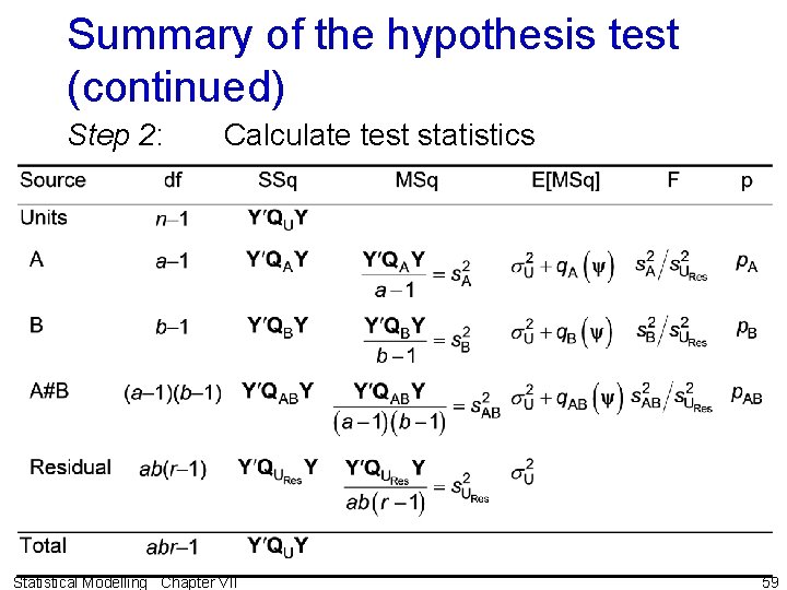
Summary of the hypothesis test (continued) Step 2: Calculate test statistics Statistical Modelling Chapter VII 59
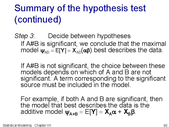
Summary of the hypothesis test (continued) Step 3: Decide between hypotheses If A#B is significant, we conclude that the maximal model y. AB = E[Y] = XAB(ab) best describes the data. If A#B is not significant, the choice between these models depends on which of A and B are not significant. A term corresponding to the significant source must be included in the model. For example, if both A and B are significant, then the model that best describes the data is the additive model y. A+B = E[Y] = XAa + XBb. Statistical Modelling Chapter VII 60
f) Computation of ANOVA and diagnostic checking in R • The assumptions underlying a factorial experiment will be the same as for the basic design employed, except that residuals-versus-factor plots of residuals are also produced for all the factors in the experiment. Statistical Modelling Chapter VII 61
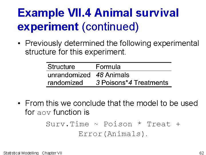
Example VII. 4 Animal survival experiment (continued) • Previously determined the following experimental structure for this experiment. • From this we conclude that the model to be used for aov function is Surv. Time ~ Poison * Treat + Error(Animals). Statistical Modelling Chapter VII 62
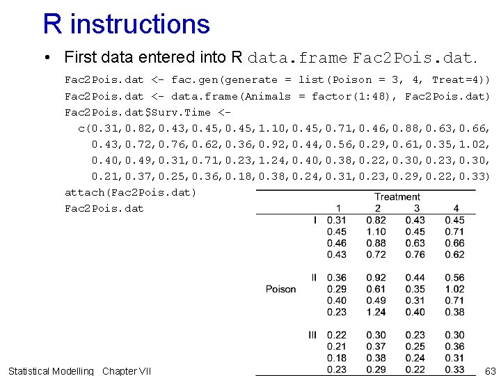
R instructions • First data entered into R data. frame Fac 2 Pois. dat <- fac. gen(generate = list(Poison = 3, 4, Treat=4)) Fac 2 Pois. dat <- data. frame(Animals = factor(1: 48), Fac 2 Pois. dat) Fac 2 Pois. dat$Surv. Time <c(0. 31, 0. 82, 0. 43, 0. 45, 1. 10, 0. 45, 0. 71, 0. 46, 0. 88, 0. 63, 0. 66, 0. 43, 0. 72, 0. 76, 0. 62, 0. 36, 0. 92, 0. 44, 0. 56, 0. 29, 0. 61, 0. 35, 1. 02, 0. 40, 0. 49, 0. 31, 0. 71, 0. 23, 1. 24, 0. 40, 0. 38, 0. 22, 0. 30, 0. 23, 0. 30, 0. 21, 0. 37, 0. 25, 0. 36, 0. 18, 0. 38, 0. 24, 0. 31, 0. 23, 0. 29, 0. 22, 0. 33) attach(Fac 2 Pois. dat) Fac 2 Pois. dat Statistical Modelling Chapter VII 63
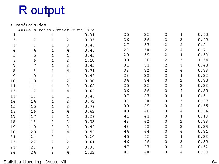
R output > Fac 2 Pois. dat Animals Poison Treat Surv. Time 1 1 0. 31 2 2 1 2 0. 82 3 3 1 3 0. 43 4 4 1 4 0. 45 5 5 1 1 0. 45 6 6 1 2 1. 10 7 7 1 3 0. 45 8 8 1 4 0. 71 9 9 1 1 0. 46 10 10 1 2 0. 88 11 11 1 3 0. 63 12 12 1 4 0. 66 13 13 1 1 0. 43 14 14 1 2 0. 72 15 15 1 3 0. 76 16 16 1 4 0. 62 17 17 2 1 0. 36 18 18 2 2 0. 92 19 19 2 3 0. 44 20 20 2 4 0. 56 21 21 2 1 0. 29 22 22 2 2 0. 61 23 23 2 3 0. 35 24 24 2 4 1. 02 Statistical Modelling Chapter VII 25 26 27 28 29 30 31 32 33 34 35 36 37 38 39 40 41 42 43 44 45 46 47 48 2 2 2 2 3 3 3 3 1 2 3 4 1 2 3 4 0. 40 0. 49 0. 31 0. 71 0. 23 1. 24 0. 40 0. 38 0. 22 0. 30 0. 23 0. 30 0. 21 0. 37 0. 25 0. 36 0. 18 0. 38 0. 24 0. 31 0. 23 0. 29 0. 22 0. 33 64
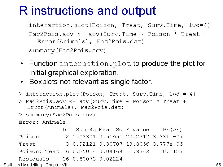
R instructions and output interaction. plot(Poison, Treat, Surv. Time, lwd=4) Fac 2 Pois. aov <- aov(Surv. Time ~ Poison * Treat + Error(Animals), Fac 2 Pois. dat) summary(Fac 2 Pois. aov) • Function interaction. plot to produce the plot for initial graphical exploration. • Boxplots not relevant as single factor. > interaction. plot(Poison, Treat, Surv. Time, lwd = 4) > Fac 2 Pois. aov <- aov(Surv. Time ~ Poison * Treat + Error(Animals), Fac 2 Pois. dat) > summary(Fac 2 Pois. aov) Error: Animals Df Sum Sq Mean Sq F value Pr(>F) Poison 2 1. 03301 0. 51651 23. 2217 3. 331 e-07 Treat 3 0. 92121 0. 30707 13. 8056 3. 777 e-06 Poison: Treat 6 0. 25014 0. 04169 1. 8743 0. 1123 Residuals 36 0. 80073 0. 02224 Statistical Modelling Chapter VII 65
Diagnostic checking • As experiment was set up as a CRD, the assumptions underlying its analysis will be the same as for the CRD • Diagnostic checking the same — in particular, Tukey’s one-degree-of-freedom-for-nonadditivity cannot be computed. • The R output produced by the expressions that deal with diagnostic checking is as follows: > > > > > # # Diagnostic checking # res <- resid. errors(Fac 2 Pois. aov) fit <- fitted. errors(Fac 2 Pois. aov) plot(fit, res, pch=16) plot(as. numeric(Poison), res, pch=16) plot(as. numeric(Treat), res, pch=16) qqnorm(res, pch=16) qqline(res) Statistical Modelling Chapter VII 66
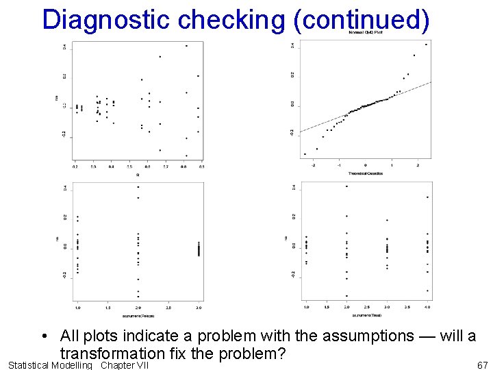
Diagnostic checking (continued) • All plots indicate a problem with the assumptions — will a transformation fix the problem? Statistical Modelling Chapter VII 67
g) Box-Cox transformations for correcting transformable non-additivity • Box, Hunter and Hunter (sec. 7. 9) describe the Box-Cox procedure for determining the appropriate power transformation for a set of data. • It has been implemented in the R function boxcox supplied in the MASS library that comes with R. • When you run this procedure you obtain a plot of the log-likelihood of l, the power of the transformation to be used (for l = 0 use the ln transformation). • However, the function does not work with aovlist objects and so the aov function must be repeated without the Error function. Statistical Modelling Chapter VII 68
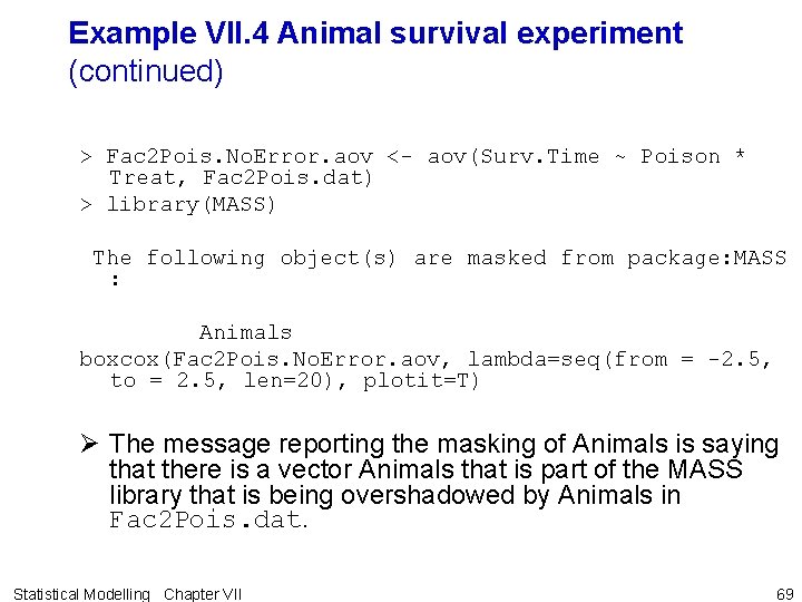
Example VII. 4 Animal survival experiment (continued) > Fac 2 Pois. No. Error. aov <- aov(Surv. Time ~ Poison * Treat, Fac 2 Pois. dat) > library(MASS) The following object(s) are masked from package: MASS : Animals boxcox(Fac 2 Pois. No. Error. aov, lambda=seq(from = -2. 5, to = 2. 5, len=20), plotit=T) Ø The message reporting the masking of Animals is saying that there is a vector Animals that is part of the MASS library that is being overshadowed by Animals in Fac 2 Pois. dat. Statistical Modelling Chapter VII 69
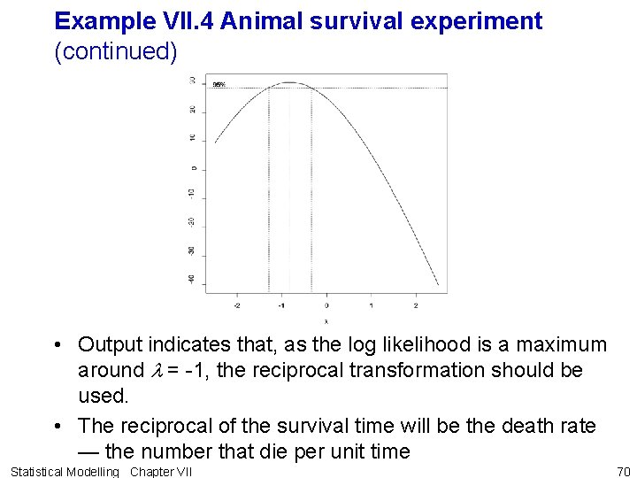
Example VII. 4 Animal survival experiment (continued) • Output indicates that, as the log likelihood is a maximum around l = -1, the reciprocal transformation should be used. • The reciprocal of the survival time will be the death rate — the number that die per unit time Statistical Modelling Chapter VII 70
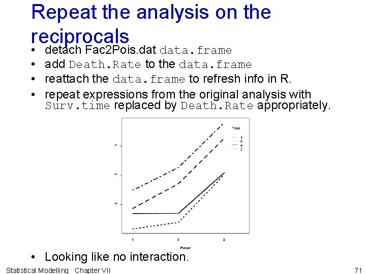
Repeat the analysis on the reciprocals • • detach Fac 2 Pois. data. frame add Death. Rate to the data. frame reattach the data. frame to refresh info in R. repeat expressions from the original analysis with Surv. time replaced by Death. Rate appropriately. • Looking like no interaction. Statistical Modelling Chapter VII 71
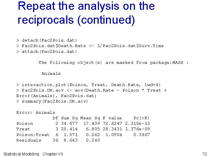
Repeat the analysis on the reciprocals (continued) > detach(Fac 2 Pois. dat) > Fac 2 Pois. dat$Death. Rate <- 1/Fac 2 Pois. dat$Surv. Time > attach(Fac 2 Pois. dat) The following object(s) are masked from package: MASS : Animals > interaction. plot(Poison, Treat, Death. Rate, lwd=4) > Fac 2 Pois. DR. aov <- aov(Death. Rate ~ Poison * Treat + Error(Animals), Fac 2 Pois. dat) > summary(Fac 2 Pois. DR. aov) Error: Animals Df Sum Sq Mean Sq F value Pr(>F) Poison 2 34. 877 17. 439 72. 6347 2. 310 e-13 Treat 3 20. 414 6. 805 28. 3431 1. 376 e-09 Poison: Treat 6 1. 571 0. 262 1. 0904 0. 3867 Residuals 36 8. 643 0. 240 Statistical Modelling Chapter VII 72
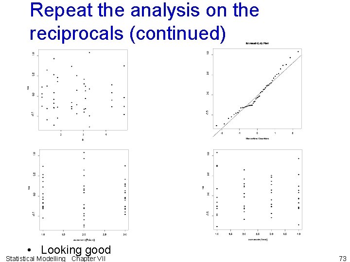
Repeat the analysis on the reciprocals (continued) • Looking good Statistical Modelling Chapter VII 73
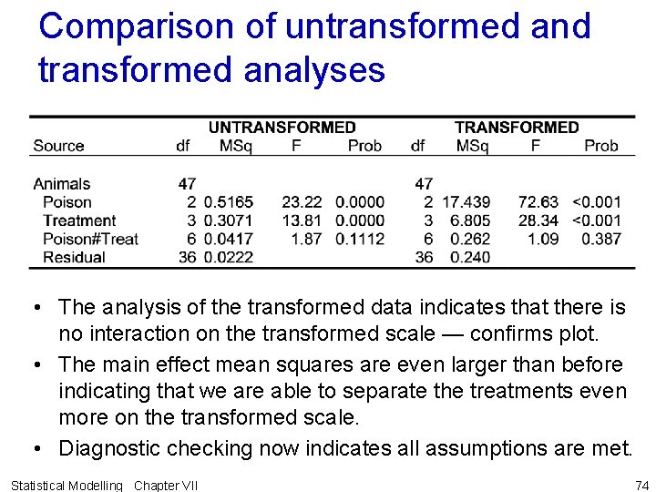
Comparison of untransformed and transformed analyses • The analysis of the transformed data indicates that there is no interaction on the transformed scale — confirms plot. • The main effect mean squares are even larger than before indicating that we are able to separate the treatments even more on the transformed scale. • Diagnostic checking now indicates all assumptions are met. Statistical Modelling Chapter VII 74
VII. F Treatment differences • As usual the examination of treatment differences can be based on multiple comparisons or submodels. Statistical Modelling Chapter VII 75
a) Multiple comparison procedures • For two factor experiments, there will be altogether three tables of means, namely one for each of A, B and A B. • Which table is of interest depends on the results of the hypothesis tests outlined above. • However, in all cases Tukey’s HSD procedure will be employed to determine which means are significantly different. Statistical Modelling Chapter VII 76
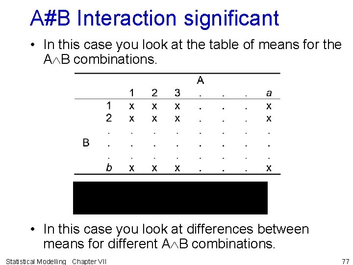
A#B Interaction significant • In this case you look at the table of means for the A B combinations. • In this case you look at differences between means for different A B combinations. Statistical Modelling Chapter VII 77
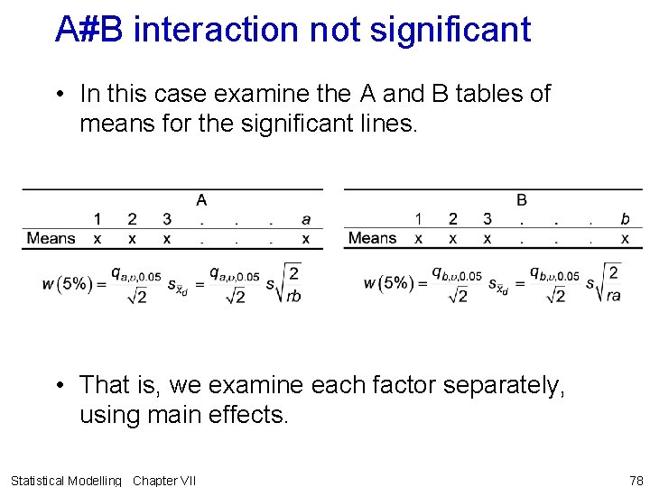
A#B interaction not significant • In this case examine the A and B tables of means for the significant lines. • That is, we examine each factor separately, using main effects. Statistical Modelling Chapter VII 78
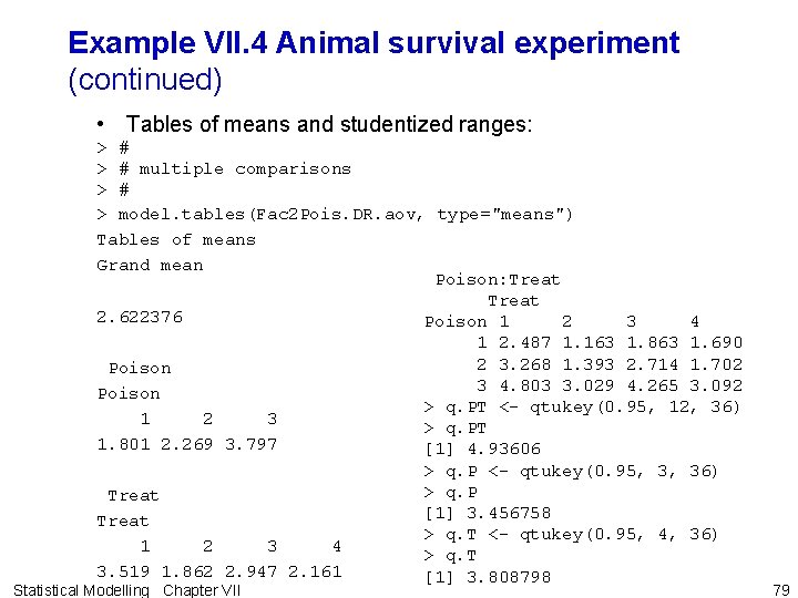
Example VII. 4 Animal survival experiment (continued) • Tables of means and studentized ranges: > # multiple comparisons > # > model. tables(Fac 2 Pois. DR. aov, type="means") Tables of means Grand mean Poison: Treat 2. 622376 Poison 1 2 3 4 1 2. 487 1. 163 1. 863 1. 690 2 3. 268 1. 393 2. 714 1. 702 Poison 3 4. 803 3. 029 4. 265 3. 092 Poison > q. PT <- qtukey(0. 95, 12, 36) 1 2 3 > q. PT 1. 801 2. 269 3. 797 [1] 4. 93606 > q. P <- qtukey(0. 95, 3, 36) > q. P Treat [1] 3. 456758 Treat > q. T <- qtukey(0. 95, 4, 36) 1 2 3 4 > q. T 3. 519 1. 862 2. 947 2. 161 [1] 3. 808798 Statistical Modelling Chapter VII 79
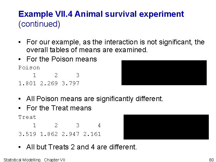
Example VII. 4 Animal survival experiment (continued) • For our example, as the interaction is not significant, the overall tables of means are examined. • For the Poison means Poison 1 2 3 1. 801 2. 269 3. 797 • All Poison means are significantly different. • For the Treat means Treat 1 2 3 4 3. 519 1. 862 2. 947 2. 161 • All but Treats 2 and 4 are different. Statistical Modelling Chapter VII 80
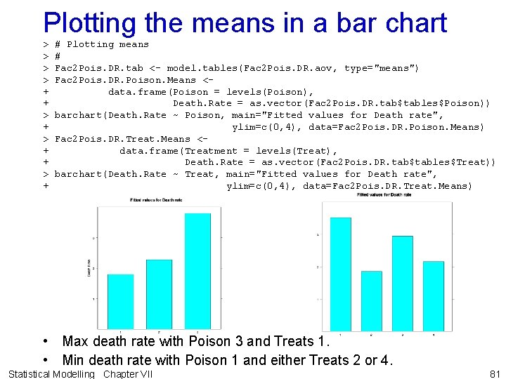
Plotting the means in a bar chart > > + + > + # Plotting means # Fac 2 Pois. DR. tab <- model. tables(Fac 2 Pois. DR. aov, type="means") Fac 2 Pois. DR. Poison. Means <data. frame(Poison = levels(Poison), Death. Rate = as. vector(Fac 2 Pois. DR. tab$tables$Poison)) barchart(Death. Rate ~ Poison, main="Fitted values for Death rate", ylim=c(0, 4), data=Fac 2 Pois. DR. Poison. Means) Fac 2 Pois. DR. Treat. Means <data. frame(Treatment = levels(Treat), Death. Rate = as. vector(Fac 2 Pois. DR. tab$tables$Treat)) barchart(Death. Rate ~ Treat, main="Fitted values for Death rate", ylim=c(0, 4), data=Fac 2 Pois. DR. Treat. Means) • Max death rate with Poison 3 and Treats 1. • Min death rate with Poison 1 and either Treats 2 or 4. Statistical Modelling Chapter VII 81
If interaction significant, 2 possibilities • Possible researcher’s objective(s): i. finding levels combination(s) of the factors that maximize (or minimize) response variable or describing response variable differences between all levels combinations of the factors ii. for each level of one factor, finding the level of the other factor that maximizes (or minimizes) the response variable or describing the response variable differences between the levels of the other factor iii. finding a level of one factor for which there is no difference between the levels of the other factor • For i: examine all possible pairs of differences between all means. • For ii & iii: examine pairs of mean differences between levels of one factor for each level of other factor i. e. in slices for each level of other factor (= examining simple effects). Statistical Modelling Chapter VII 82
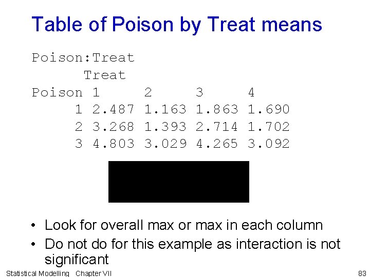
Table of Poison by Treat means Poison: Treat Poison 1 1 2. 487 2 3. 268 3 4. 803 2 1. 163 1. 393 3. 029 3 1. 863 2. 714 4. 265 4 1. 690 1. 702 3. 092 • Look for overall max or max in each column • Do not do for this example as interaction is not significant Statistical Modelling Chapter VII 83
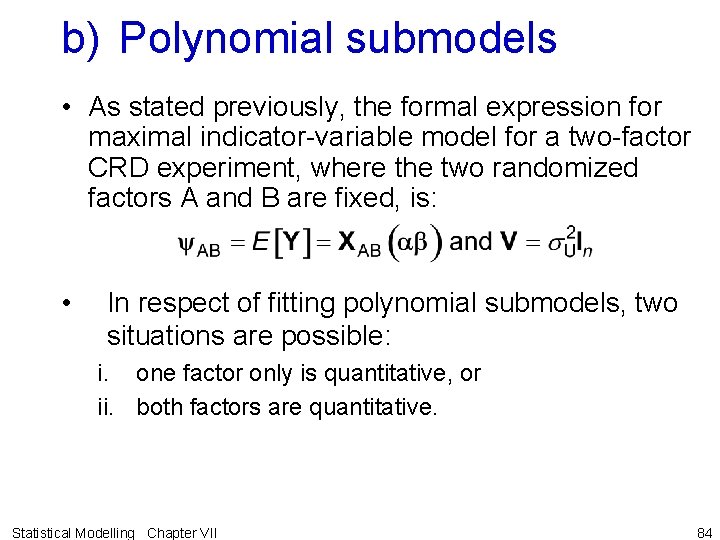
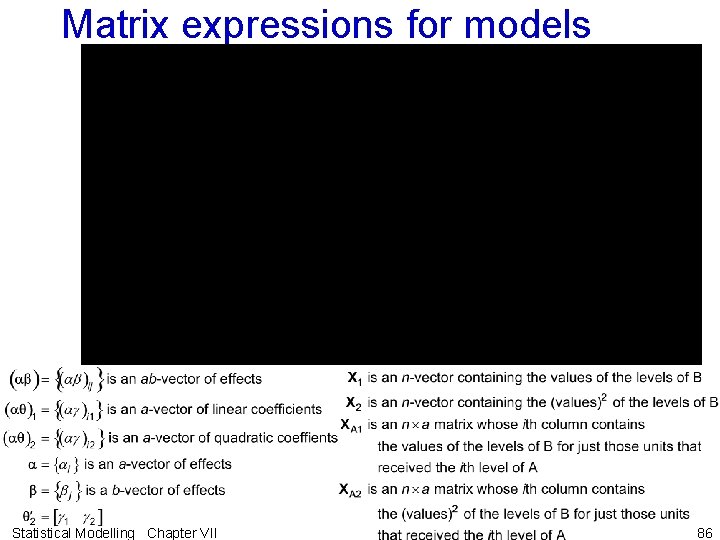
b) Polynomial submodels • As stated previously, the formal expression for maximal indicator-variable model for a two-factor CRD experiment, where the two randomized factors A and B are fixed, is: • In respect of fitting polynomial submodels, two situations are possible: i. one factor only is quantitative, or ii. both factors are quantitative. Statistical Modelling Chapter VII 84
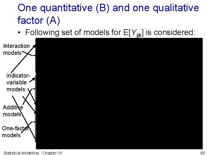
One quantitative (B) and one qualitative factor (A) • Following set of models for E[Yijk] is considered: Interaction models indicatorvariable models Additive models One-factor models Statistical Modelling Chapter VII 85
Matrix expressions for models Statistical Modelling Chapter VII 86
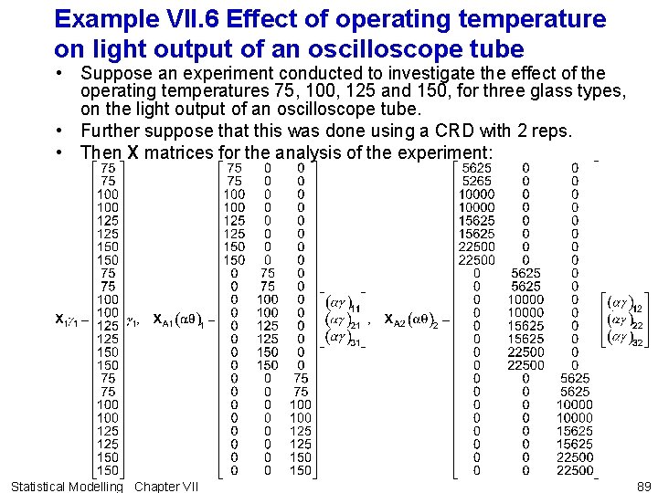
Example VII. 6 Effect of operating temperature on light output of an oscilloscope tube • Suppose an experiment conducted to investigate the effect of the operating temperatures 75, 100, 125 and 150, for three glass types, on the light output of an oscilloscope tube. • Further suppose that this was done using a CRD with 2 reps. • Then X matrices for the analysis of the experiment: Statistical Modelling Chapter VII 89
Why this set of expectation models? • As before, gs are used for the coefficients of polynomial terms – a numeric subscript for each quantitative fixed factor in the experiment is placed on the gs to indicate the degree(s) to which the factor(s) is(are) raised. • The above models are ordered from the most complex to the simplest. • They obey two rules: • Rule VII. 1: The set of expectation models corresponds to the set of all possible combinations of potential expectation terms, subject to restriction that terms marginal to another expectation term are excluded from the model; • Rule VII. 2: An expectation model must include all polynomial terms of lower degree than a polynomial term that has been put in the model. Statistical Modelling Chapter VII 90
Definitions to determine if a polynomial term is of lower degree • Definition VII. 7: A polynomial term is one in which the X matrix involves the quantitative levels of a factor(s). • Definition VII. 8: The degree for a polynomial term with respect to a quantitative factor is the power to which levels of that factor are to be raised in this term. • Definition VII. 9: A polynomial term is said to be of lower degree than a second polynomial term if, – for each quantitative factor in first term, its degree is less than or equal to its degree in the second term and – the degree of at least one factor in the first term is less than that of the same factor in the second term. Statistical Modelling Chapter VII 91
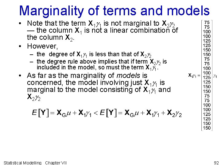
Marginality of terms and models • Note that the term X 1 g 1 is not marginal to X 2 g 2 — the column X 1 is not a linear combination of the column X 2. • However, – the degree of X 1 g 1 is less than that of X 2 g 2 – the degree rule above implies that if term X 2 g 2 is included in the model, so must the term X 1 g 1. • As far as the marginality of models is concerned, the model involving just X 1 g 1 is marginal to the model consisting of X 1 g 1 and X 2 g 2 Statistical Modelling Chapter VII 92
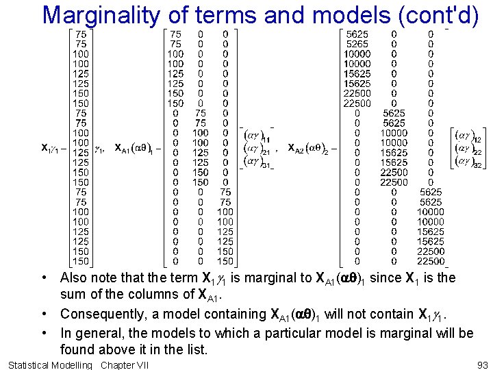
Marginality of terms and models (cont'd) • Also note that the term X 1 g 1 is marginal to XA 1(aq)1 since X 1 is the sum of the columns of XA 1. • Consequently, a model containing XA 1(aq)1 will not contain X 1 g 1. • In general, the models to which a particular model is marginal will be found above it in the list. Statistical Modelling Chapter VII 93
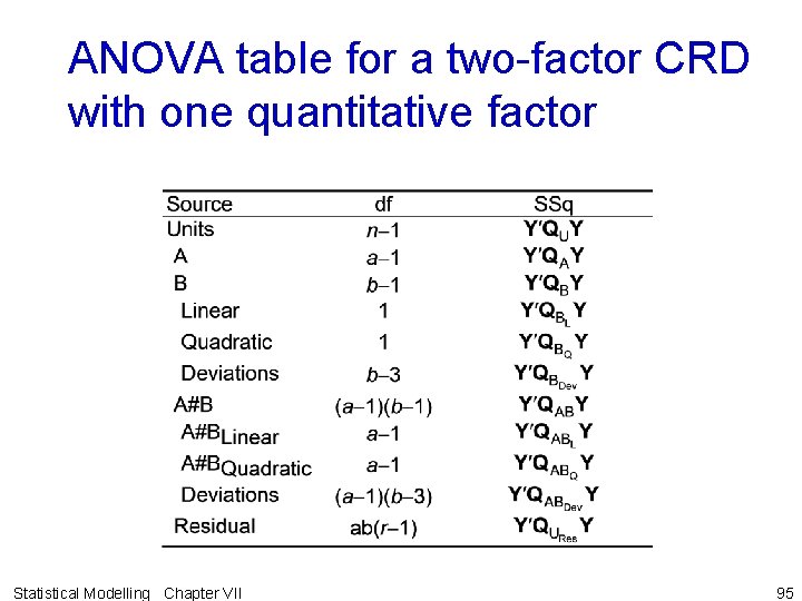
ANOVA table for a two-factor CRD with one quantitative factor Statistical Modelling Chapter VII 95
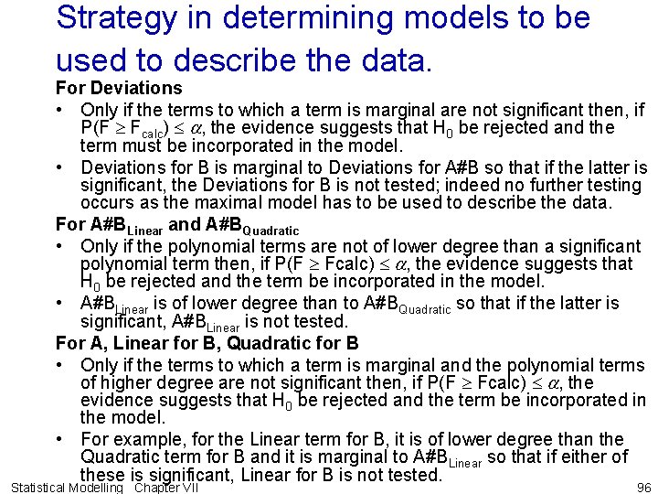
Strategy in determining models to be used to describe the data. For Deviations • Only if the terms to which a term is marginal are not significant then, if P(F Fcalc) a, the evidence suggests that H 0 be rejected and the term must be incorporated in the model. • Deviations for B is marginal to Deviations for A#B so that if the latter is significant, the Deviations for B is not tested; indeed no further testing occurs as the maximal model has to be used to describe the data. For A#BLinear and A#BQuadratic • Only if the polynomial terms are not of lower degree than a significant polynomial term then, if P(F Fcalc) a, the evidence suggests that H 0 be rejected and the term be incorporated in the model. • A#BLinear is of lower degree than to A#BQuadratic so that if the latter is significant, A#BLinear is not tested. For A, Linear for B, Quadratic for B • Only if the terms to which a term is marginal and the polynomial terms of higher degree are not significant then, if P(F Fcalc) a, the evidence suggests that H 0 be rejected and the term be incorporated in the model. • For example, for the Linear term for B, it is of lower degree than the Quadratic term for B and it is marginal to A#BLinear so that if either of these is significant, Linear for B is not tested. Statistical Modelling Chapter VII 96
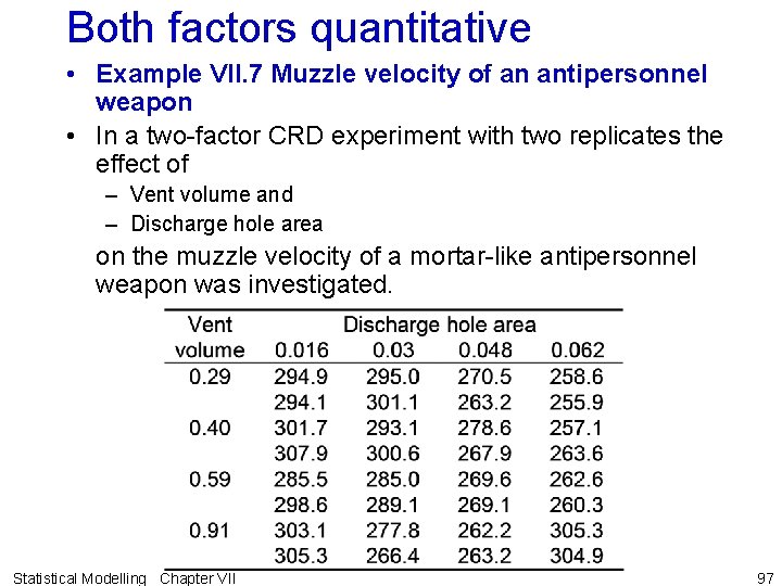
Both factors quantitative • Example VII. 7 Muzzle velocity of an antipersonnel weapon • In a two-factor CRD experiment with two replicates the effect of – Vent volume and – Discharge hole area on the muzzle velocity of a mortar-like antipersonnel weapon was investigated. Statistical Modelling Chapter VII 97
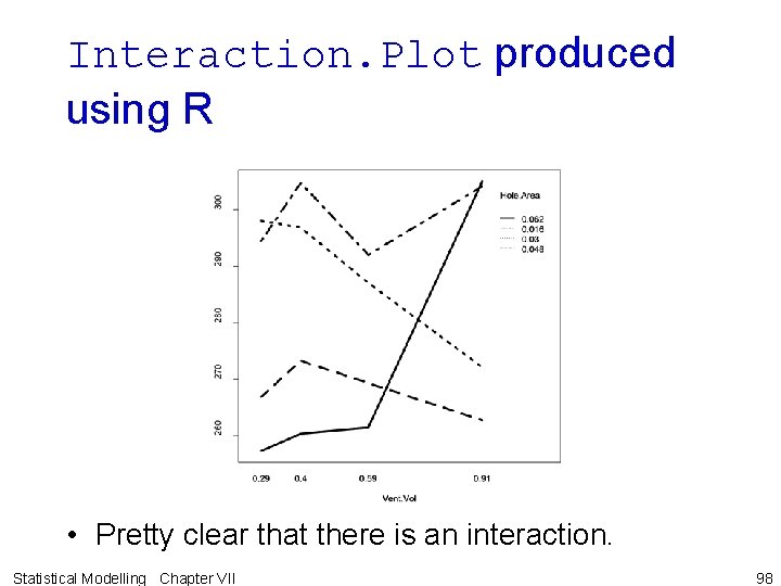
Interaction. Plot produced using R • Pretty clear that there is an interaction. Statistical Modelling Chapter VII 98
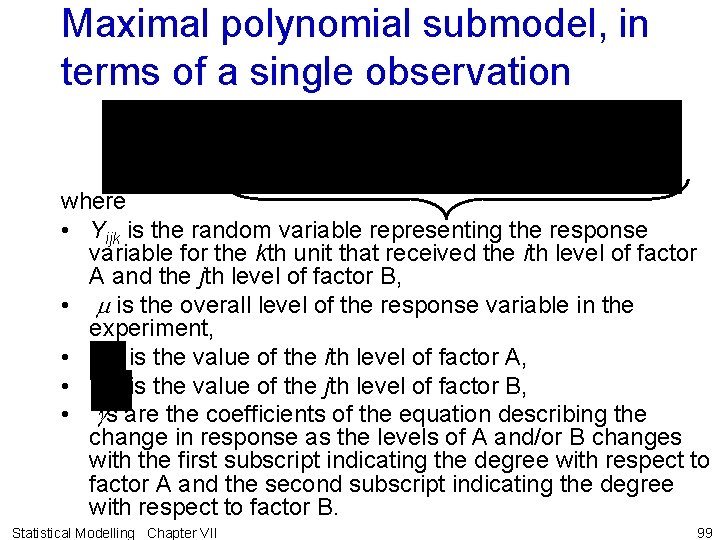
Maximal polynomial submodel, in terms of a single observation where • Yijk is the random variable representing the response variable for the kth unit that received the ith level of factor A and the jth level of factor B, • m is the overall level of the response variable in the experiment, • is the value of the ith level of factor A, • is the value of the jth level of factor B, • gs are the coefficients of the equation describing the change in response as the levels of A and/or B changes with the first subscript indicating the degree with respect to factor A and the second subscript indicating the degree with respect to factor B. Statistical Modelling Chapter VII 99

Maximal polynomial submodel, in matrix terms • X is an n 8 matrix whose columns are the products of the values of the levels of A and B as indicated by the subscripts in X. • For example – 3 rd column consists of the values of the levels of B – 7 th column the product of the squared values of the levels of A with the values of the levels of B. Statistical Modelling Chapter VII 100
Set of expectation models considered when both factors are quantitative nonsmooth A nonsmooth B Statistical Modelling Chapter VII 101
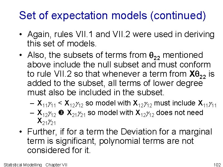
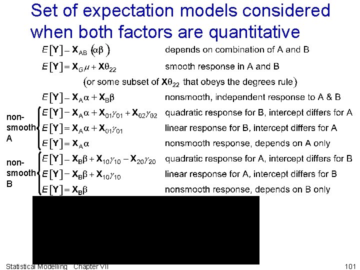
Set of expectation models (continued) • Again, rules VII. 1 and VII. 2 were used in deriving this set of models. • Also, the subsets of terms from q 22 mentioned above include the null subset and must conform to rule VII. 2 so that whenever a term from Xq 22 is added to the subset, all terms of lower degree must also be included in the subset. – X 11 g 11 < X 12 g 12 so model with X 12 g 12 must include X 11 g 11 – X 12 g 12 X 21 g 21 so model with X 12 g 12 does not need X 21 g 21 • Further, if for a term the Deviation for a marginal term is significant, polynomial terms are not considered for it. Statistical Modelling Chapter VII 102
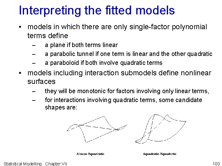
Interpreting the fitted models • models in which there are only single-factor polynomial terms define – – – a plane if both terms linear a parabolic tunnel if one term is linear and the other quadratic a paraboloid if both involve quadratic terms • models including interaction submodels define nonlinear surfaces – – they will be monotonic for factors involving only linear terms, for interactions involving quadratic terms, some candidate shapes are: Statistical Modelling Chapter VII 103
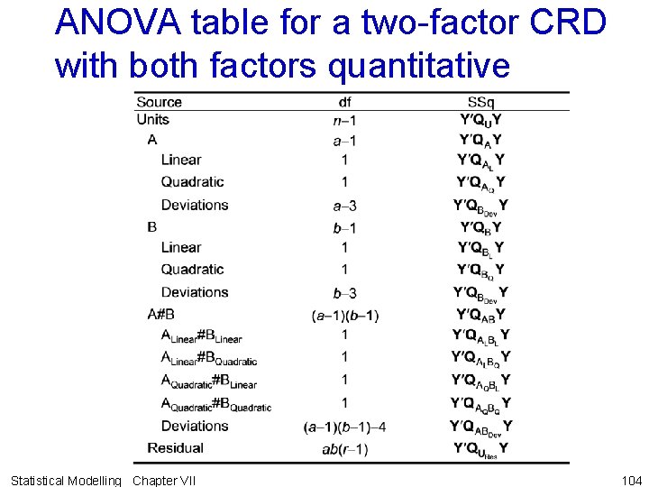
ANOVA table for a two-factor CRD with both factors quantitative Statistical Modelling Chapter VII 104
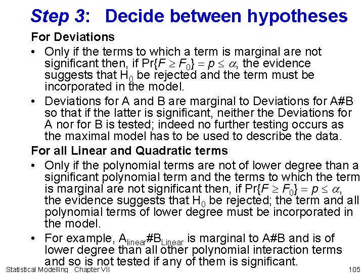
Step 3: Decide between hypotheses For Deviations • Only if the terms to which a term is marginal are not significant then, if Pr{F F 0} = p a, the evidence suggests that H 0 be rejected and the term must be incorporated in the model. • Deviations for A and B are marginal to Deviations for A#B so that if the latter is significant, neither the Deviations for A nor for B is tested; indeed no further testing occurs as the maximal model has to be used to describe the data. For all Linear and Quadratic terms • Only if the polynomial terms are not of lower degree than a significant polynomial term and the terms to which the term is marginal are not significant then, if Pr{F F 0} = p a, the evidence suggests that H 0 be rejected; the term and all polynomial terms of lower degree must be incorporated in the model. • For example, Alinear#BLinear is marginal to A#B and is of lower degree than all other polynomial interaction terms and so is not tested if any of them is significant. Statistical Modelling Chapter VII 105
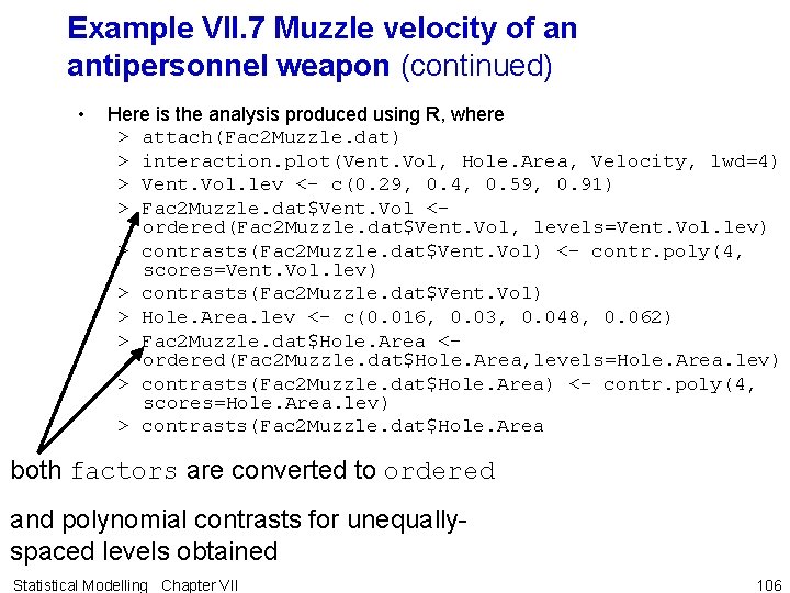
Example VII. 7 Muzzle velocity of an antipersonnel weapon (continued) • Here is the analysis produced using R, where > attach(Fac 2 Muzzle. dat) > interaction. plot(Vent. Vol, Hole. Area, Velocity, lwd=4) > Vent. Vol. lev <- c(0. 29, 0. 4, 0. 59, 0. 91) > Fac 2 Muzzle. dat$Vent. Vol <ordered(Fac 2 Muzzle. dat$Vent. Vol, levels=Vent. Vol. lev) > contrasts(Fac 2 Muzzle. dat$Vent. Vol) <- contr. poly(4, scores=Vent. Vol. lev) > contrasts(Fac 2 Muzzle. dat$Vent. Vol) > Hole. Area. lev <- c(0. 016, 0. 03, 0. 048, 0. 062) > Fac 2 Muzzle. dat$Hole. Area <ordered(Fac 2 Muzzle. dat$Hole. Area, levels=Hole. Area. lev) > contrasts(Fac 2 Muzzle. dat$Hole. Area) <- contr. poly(4, scores=Hole. Area. lev) > contrasts(Fac 2 Muzzle. dat$Hole. Area both factors are converted to ordered and polynomial contrasts for unequallyspaced levels obtained Statistical Modelling Chapter VII 106
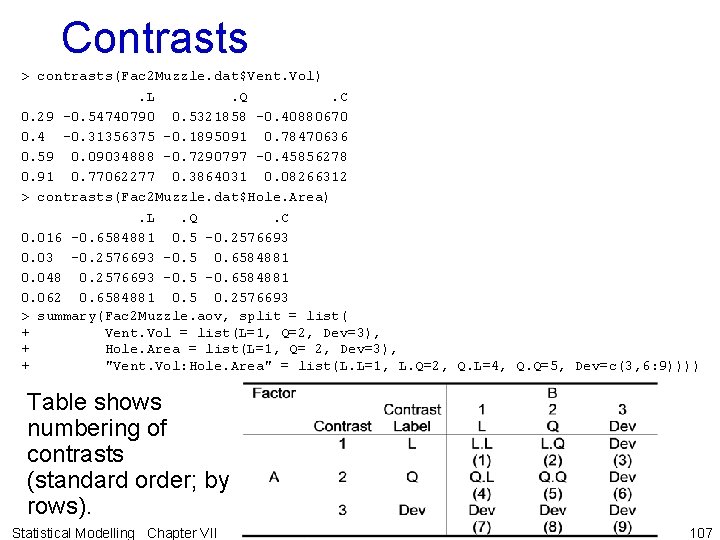
Contrasts > contrasts(Fac 2 Muzzle. dat$Vent. Vol). L. Q. C 0. 29 -0. 54740790 0. 5321858 -0. 40880670 0. 4 -0. 31356375 -0. 1895091 0. 78470636 0. 59 0. 09034888 -0. 7290797 -0. 45856278 0. 91 0. 77062277 0. 3864031 0. 08266312 > contrasts(Fac 2 Muzzle. dat$Hole. Area). L. Q. C 0. 016 -0. 6584881 0. 5 -0. 2576693 0. 03 -0. 2576693 -0. 5 0. 6584881 0. 048 0. 2576693 -0. 5 -0. 6584881 0. 062 0. 6584881 0. 5 0. 2576693 > summary(Fac 2 Muzzle. aov, split = list( + Vent. Vol = list(L=1, Q=2, Dev=3), + Hole. Area = list(L=1, Q= 2, Dev=3), + "Vent. Vol: Hole. Area" = list(L. L=1, L. Q=2, Q. L=4, Q. Q=5, Dev=c(3, 6: 9)))) Table shows numbering of contrasts (standard order; by rows). Statistical Modelling Chapter VII 107
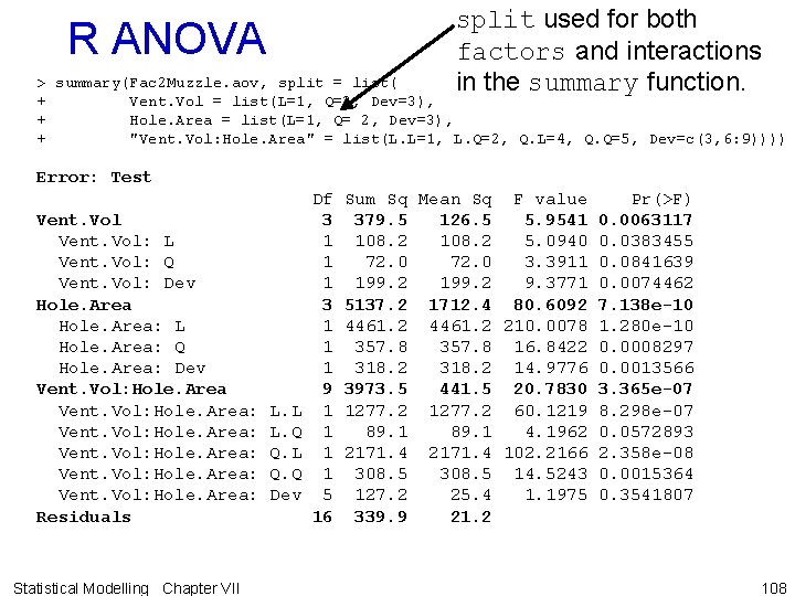
split used for both factors and interactions in the summary function. R ANOVA > summary(Fac 2 Muzzle. aov, split = list( + Vent. Vol = list(L=1, Q=2, Dev=3), + Hole. Area = list(L=1, Q= 2, Dev=3), + "Vent. Vol: Hole. Area" = list(L. L=1, L. Q=2, Q. L=4, Q. Q=5, Dev=c(3, 6: 9)))) Error: Test Vent. Vol: L Vent. Vol: Q Vent. Vol: Dev Hole. Area: L Hole. Area: Q Hole. Area: Dev Vent. Vol: Hole. Area: Residuals Statistical Modelling Chapter VII L. L L. Q Q. L Q. Q Dev Df 3 1 1 1 9 1 1 5 16 Sum Sq Mean Sq F value Pr(>F) 379. 5 126. 5 5. 9541 0. 0063117 108. 2 5. 0940 0. 0383455 72. 0 3. 3911 0. 0841639 199. 2 9. 3771 0. 0074462 5137. 2 1712. 4 80. 6092 7. 138 e-10 4461. 2 210. 0078 1. 280 e-10 357. 8 16. 8422 0. 0008297 318. 2 14. 9776 0. 0013566 3973. 5 441. 5 20. 7830 3. 365 e-07 1277. 2 60. 1219 8. 298 e-07 89. 1 4. 1962 0. 0572893 2171. 4 102. 2166 2. 358 e-08 308. 5 14. 5243 0. 0015364 127. 2 25. 4 1. 1975 0. 3541807 339. 9 21. 2 108
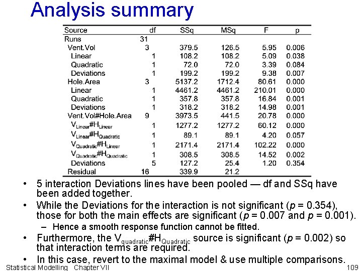
Analysis summary • 5 interaction Deviations lines have been pooled — df and SSq have been added together. • While the Deviations for the interaction is not significant (p = 0. 354), those for both the main effects are significant (p = 0. 007 and p = 0. 001). – Hence a smooth response function cannot be fitted. • Furthermore, the Vquadratic#HQuadratic source is significant (p = 0. 002) so that interaction terms are required. • In this case, revert to the maximal model & use multiple comparisons. Statistical Modelling Chapter VII 109
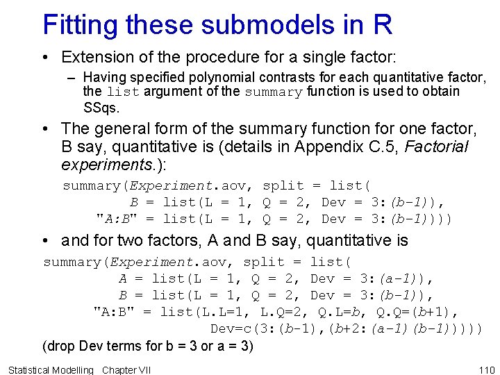
Fitting these submodels in R • Extension of the procedure for a single factor: – Having specified polynomial contrasts for each quantitative factor, the list argument of the summary function is used to obtain SSqs. • The general form of the summary function for one factor, B say, quantitative is (details in Appendix C. 5, Factorial experiments. ): summary(Experiment. aov, split = list( B = list(L = 1, Q = 2, Dev = 3: (b-1)), "A: B" = list(L = 1, Q = 2, Dev = 3: (b-1)))) • and for two factors, A and B say, quantitative is summary(Experiment. aov, split = list( A = list(L = 1, Q = 2, Dev = 3: (a-1)), B = list(L = 1, Q = 2, Dev = 3: (b-1)), "A: B" = list(L. L=1, L. Q=2, Q. L=b, Q. Q=(b+1), Dev=c(3: (b-1), (b+2: (a-1)(b-1))))) (drop Dev terms for b = 3 or a = 3) Statistical Modelling Chapter VII 110
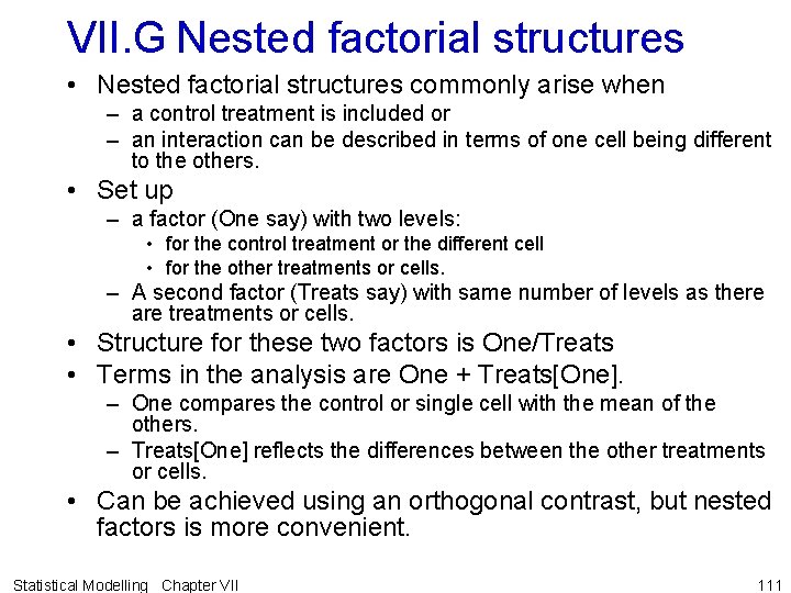
VII. G Nested factorial structures • Nested factorial structures commonly arise when – a control treatment is included or – an interaction can be described in terms of one cell being different to the others. • Set up – a factor (One say) with two levels: • for the control treatment or the different cell • for the other treatments or cells. – A second factor (Treats say) with same number of levels as there are treatments or cells. • Structure for these two factors is One/Treats • Terms in the analysis are One + Treats[One]. – One compares the control or single cell with the mean of the others. – Treats[One] reflects the differences between the other treatments or cells. • Can be achieved using an orthogonal contrast, but nested factors is more convenient. Statistical Modelling Chapter VII 111
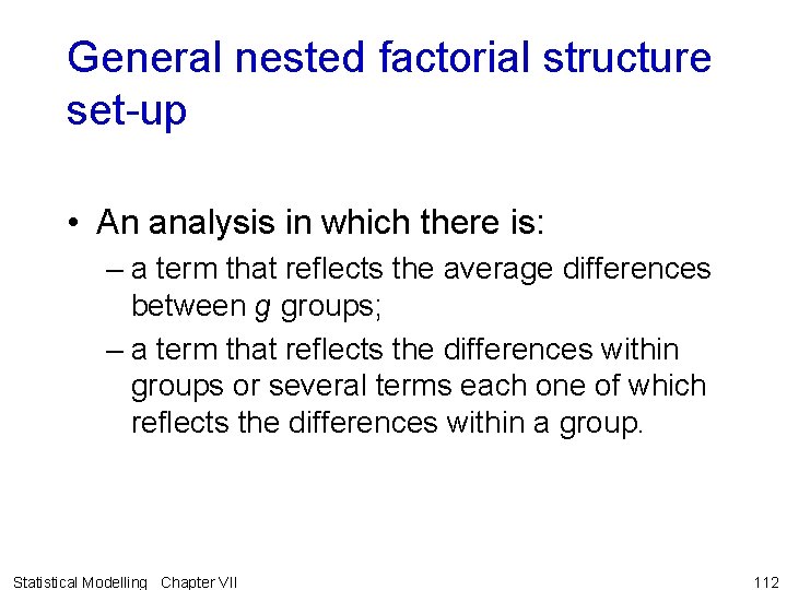
General nested factorial structure set-up • An analysis in which there is: – a term that reflects the average differences between g groups; – a term that reflects the differences within groups or several terms each one of which reflects the differences within a group. Statistical Modelling Chapter VII 112
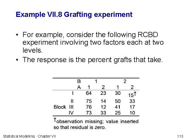
Example VII. 8 Grafting experiment • For example, consider the following RCBD experiment involving two factors each at two levels. • The response is the percent grafts that take. Statistical Modelling Chapter VII 113
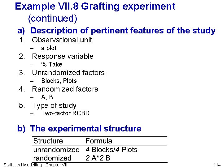
Example VII. 8 Grafting experiment (continued) a) Description of pertinent features of the study 1. Observational unit – a plot 2. Response variable – % Take 3. Unrandomized factors – Blocks, Plots 4. Randomized factors – A, B 5. Type of study – Two-factor RCBD b) The experimental structure Statistical Modelling Chapter VII 114
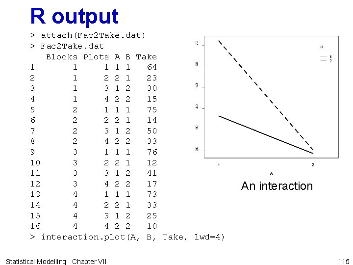
R output > attach(Fac 2 Take. dat) > Fac 2 Take. dat Blocks Plots A B Take 1 1 1 64 2 1 23 3 1 2 30 4 1 4 2 2 15 5 2 1 1 1 75 6 2 2 2 1 14 7 2 3 1 2 50 8 2 4 2 2 33 9 3 1 1 1 76 10 3 2 2 1 12 11 3 3 1 2 41 12 3 4 2 2 17 13 4 1 1 1 73 14 4 2 2 1 33 15 4 3 1 2 25 16 4 4 2 2 10 > interaction. plot(A, B, Take, lwd=4) Statistical Modelling Chapter VII An interaction 115
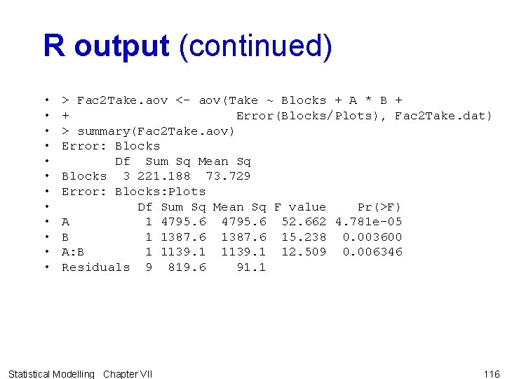
R output (continued) • • • > Fac 2 Take. aov <- aov(Take ~ Blocks + A * B + + Error(Blocks/Plots), Fac 2 Take. dat) > summary(Fac 2 Take. aov) Error: Blocks Df Sum Sq Mean Sq Blocks 3 221. 188 73. 729 Error: Blocks: Plots Df Sum Sq Mean Sq F value Pr(>F) A 1 4795. 6 52. 662 4. 781 e-05 B 1 1387. 6 15. 238 0. 003600 A: B 1 1139. 1 12. 509 0. 006346 Residuals 9 819. 6 91. 1 Statistical Modelling Chapter VII 116
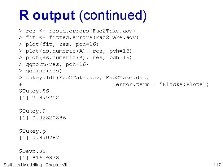
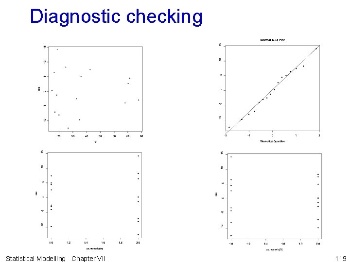
R output (continued) > res <- resid. errors(Fac 2 Take. aov) > fit <- fitted. errors(Fac 2 Take. aov) > plot(fit, res, pch=16) > plot(as. numeric(A), res, pch=16) > plot(as. numeric(B), res, pch=16) > qqnorm(res, pch=16) > qqline(res) > tukey. 1 df(Fac 2 Take. aov, Fac 2 Take. dat, + error. term = "Blocks: Plots") $Tukey. SS [1] 2. 879712 $Tukey. F [1] 0. 02820886 $Tukey. p [1] 0. 870787 $Devn. SS [1] 816. 6828 Statistical Modelling Chapter VII 117
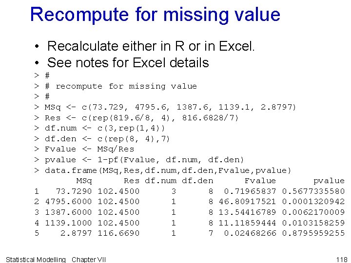
Recompute for missing value • Recalculate either in R or in Excel. • See notes for Excel details > > > > > 1 2 3 4 5 # # recompute for missing value # MSq <- c(73. 729, 4795. 6, 1387. 6, 1139. 1, 2. 8797) Res <- c(rep(819. 6/8, 4), 816. 6828/7) df. num <- c(3, rep(1, 4)) df. den <- c(rep(8, 4), 7) Fvalue <- MSq/Res pvalue <- 1 -pf(Fvalue, df. num, df. den) data. frame(MSq, Res, df. num, df. den, Fvalue, pvalue) MSq Res df. num df. den Fvalue pvalue 73. 7290 102. 4500 3 8 0. 71965837 0. 5677335580 4795. 6000 102. 4500 1 8 46. 80917521 0. 0001320942 1387. 6000 102. 4500 1 8 13. 54416789 0. 0062170009 1139. 1000 102. 4500 1 8 11. 11859444 0. 0103158259 2. 8797 116. 6690 1 7 0. 02468266 0. 8795959255 Statistical Modelling Chapter VII 118
Diagnostic checking Statistical Modelling Chapter VII 119
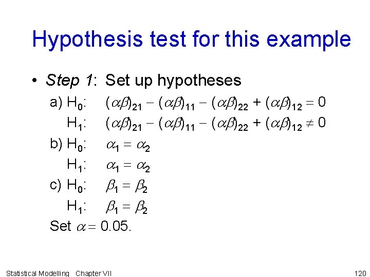
Hypothesis test for this example • Step 1: Set up hypotheses a) H 0: (ab)21 - (ab)11 - (ab)22 + (ab)12 = 0 H 1: (ab)21 - (ab)11 - (ab)22 + (ab)12 0 b) H 0: a 1 = a 2 H 1: a 1 = a 2 c) H 0: b 1 = b 2 H 1: b 1 = b 2 Set a = 0. 05. Statistical Modelling Chapter VII 120
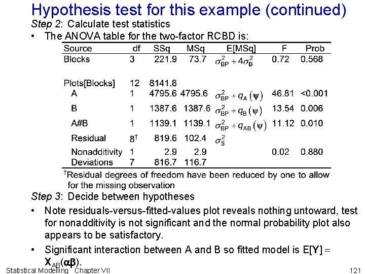
Hypothesis test for this example (continued) Step 2: Calculate test statistics • The ANOVA table for the two-factor RCBD is: Step 3: Decide between hypotheses • Note residuals-versus-fitted-values plot reveals nothing untoward, test for nonadditivity is not significant and the normal probability plot also appears to be satisfactory. • Significant interaction between A and B so fitted model is E[Y] = XAB(ab). Statistical Modelling Chapter VII 121
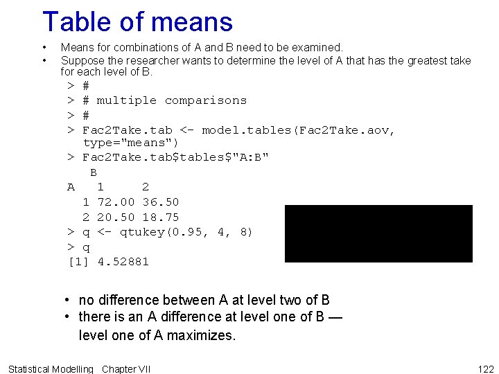
Table of means • • Means for combinations of A and B need to be examined. Suppose the researcher wants to determine the level of A that has the greatest take for each level of B. > > # # multiple comparisons # Fac 2 Take. tab <- model. tables(Fac 2 Take. aov, type="means") > Fac 2 Take. tab$tables$"A: B" B A 1 2 1 72. 00 36. 50 2 20. 50 18. 75 > q <- qtukey(0. 95, 4, 8) > q [1] 4. 52881 • no difference between A at level two of B • there is an A difference at level one of B — level one of A maximizes. Statistical Modelling Chapter VII 122
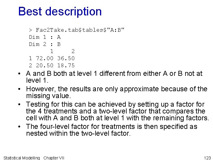
Best description > Fac 2 Take. tab$tables$"A: B" Dim 1 : A Dim 2 : B 1 2 1 72. 00 36. 50 2 20. 50 18. 75 • A and B both at level 1 different from either A or B not at level 1. • However, the results are only approximate because of the missing value. • Testing for this can be achieved by setting up a factor for the 4 treatments and a two-level factor that compares the cell with A and B both at level 1 with the remaining factors. • The four-level factor for treatments is then specified as nested within the two-level factor. Statistical Modelling Chapter VII 123
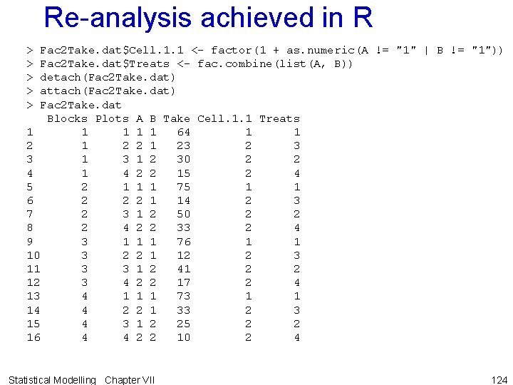
Re-analysis achieved in R > > > Fac 2 Take. dat$Cell. 1. 1 <- factor(1 + as. numeric(A != "1" | B != "1")) Fac 2 Take. dat$Treats <- fac. combine(list(A, B)) detach(Fac 2 Take. dat) attach(Fac 2 Take. dat) Fac 2 Take. dat Blocks Plots A B Take Cell. 1. 1 Treats 1 1 1 64 1 1 2 2 1 23 2 3 3 1 2 30 2 2 4 1 4 2 2 15 2 4 5 2 1 1 1 75 1 1 6 2 2 2 1 14 2 3 7 2 3 1 2 50 2 2 8 2 4 2 2 33 2 4 9 3 1 1 1 76 1 1 10 3 2 2 1 12 2 3 11 3 3 1 2 41 2 2 12 3 4 2 2 17 2 4 13 4 1 1 1 73 1 1 14 4 2 2 1 33 2 3 15 4 3 1 2 25 2 2 16 4 4 2 2 10 2 4 Statistical Modelling Chapter VII 124
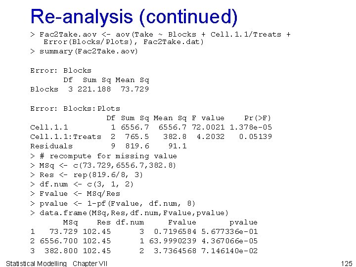
Re-analysis (continued) > Fac 2 Take. aov <- aov(Take ~ Blocks + Cell. 1. 1/Treats + Error(Blocks/Plots), Fac 2 Take. dat) > summary(Fac 2 Take. aov) Error: Blocks Df Sum Sq Mean Sq Blocks 3 221. 188 73. 729 Error: Blocks: Plots Df Sum Sq Mean Sq F value Pr(>F) Cell. 1. 1 1 6556. 7 72. 0021 1. 378 e-05 Cell. 1. 1: Treats 2 765. 5 382. 8 4. 2032 0. 05139 Residuals 9 819. 6 91. 1 > # recompute for missing value > MSq <- c(73. 729, 6556. 7, 382. 8) > Res <- rep(819. 6/8, 3) > df. num <- c(3, 1, 2) > Fvalue <- MSq/Res > pvalue <- 1 -pf(Fvalue, df. num, 8) > data. frame(MSq, Res, df. num, Fvalue, pvalue) MSq Res df. num Fvalue pvalue 1 73. 729 102. 45 3 0. 7196584 5. 677336 e-01 2 6556. 700 102. 45 1 63. 9990239 4. 367066 e-05 3 382. 800 102. 45 2 3. 7364568 7. 146140 e-02 Statistical Modelling Chapter VII 125
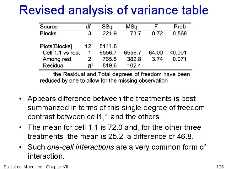
Revised analysis of variance table • Appears difference between the treatments is best summarized in terms of this single degree of freedom contrast between cell 1, 1 and the others. • The mean for cell 1, 1 is 72. 0 and, for the other three treatments, the mean is 25. 2, a difference of 46. 8. • Such one-cell interactions are a very common form of interaction. Statistical Modelling Chapter VII 126
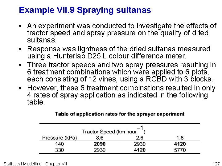
Example VII. 9 Spraying sultanas • An experiment was conducted to investigate the effects of tractor speed and spray pressure on the quality of dried sultanas. • Response was lightness of the dried sultanas measured using a Hunterlab D 25 L colour difference meter. • Three tractor speeds and two spray pressures resulting in 6 treatment combinations which were applied to 6 plots, each consisting of 12 vines, using a RCBD with 3 blocks. • However, these 6 treatment combinations resulted in only 4 rates of spray application as indicated in the following table. Statistical Modelling Chapter VII 127
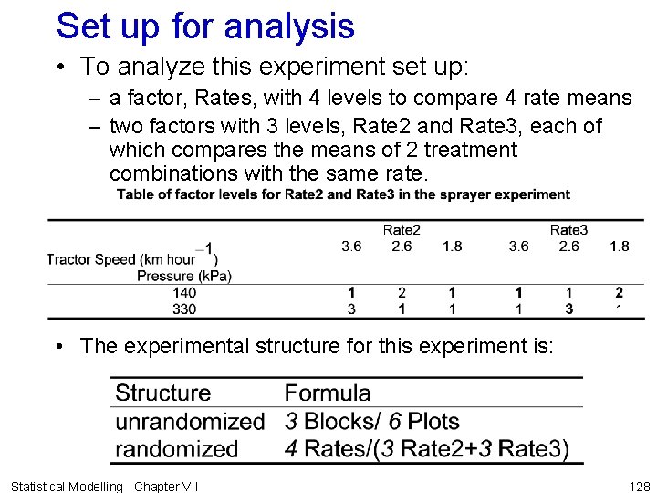
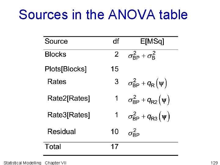
Set up for analysis • To analyze this experiment set up: – a factor, Rates, with 4 levels to compare 4 rate means – two factors with 3 levels, Rate 2 and Rate 3, each of which compares the means of 2 treatment combinations with the same rate. • The experimental structure for this experiment is: Statistical Modelling Chapter VII 128
Sources in the ANOVA table Statistical Modelling Chapter VII 129
VII. H Models and hypothesis testing for three-factor experiments • Experiment with – factors A, B and C with a, b and c levels – each of the abc combinations of A, B and C replicated r times. – n = abcr observations. • The analysis is an extension of that for a twofactor CRD. • Initial exploration using interaction plots of two factors for each level of the third factor. • use interaction. ABC. plot from the DAE library. Statistical Modelling Chapter VII 130
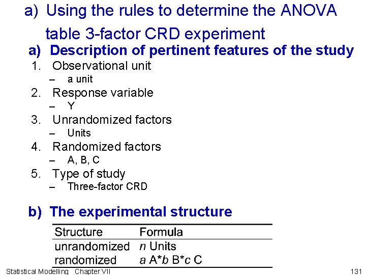
a) Using the rules to determine the ANOVA table 3 -factor CRD experiment a) Description of pertinent features of the study 1. Observational unit – a unit 2. Response variable – Y 3. Unrandomized factors – Units 4. Randomized factors – A, B, C 5. Type of study – Three-factor CRD b) The experimental structure Statistical Modelling Chapter VII 131
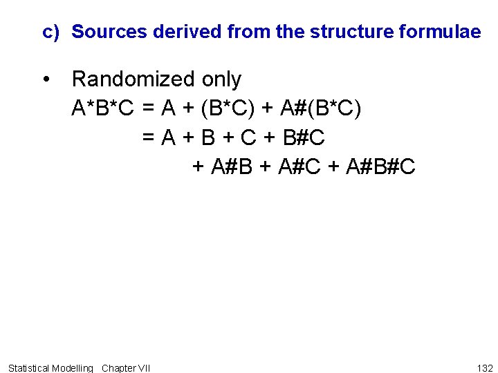
c) Sources derived from the structure formulae • Randomized only A*B*C = A + (B*C) + A#(B*C) = A + B + C + B#C + A#B + A#C + A#B#C Statistical Modelling Chapter VII 132

d) Degrees of freedom and sums of squares • The df can be derived by the cross product rule. – For each factor in the term, calculate the number of levels minus one and multiply these together. Statistical Modelling Chapter VII 133
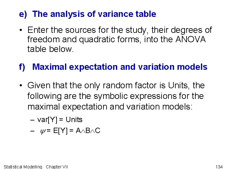
e) The analysis of variance table • Enter the sources for the study, their degrees of freedom and quadratic forms, into the ANOVA table below. f) Maximal expectation and variation models • Given that the only random factor is Units, the following are the symbolic expressions for the maximal expectation and variation models: – var[Y] = Units – y = E[Y] = A B C Statistical Modelling Chapter VII 134
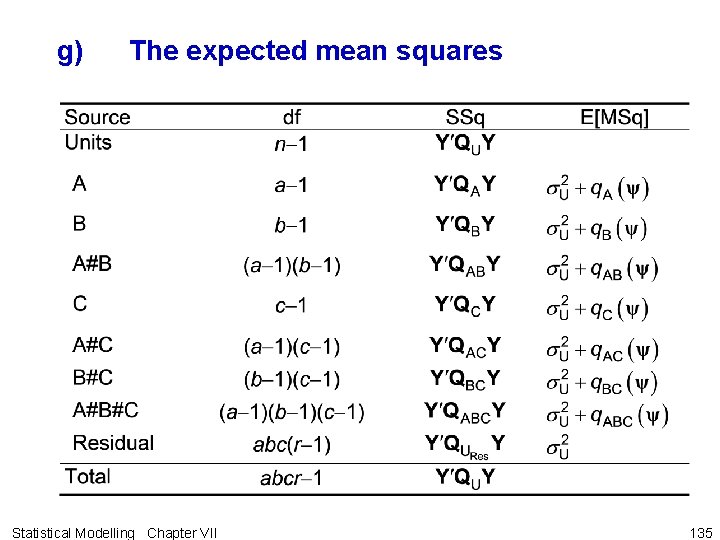
g) The expected mean squares Statistical Modelling Chapter VII 135
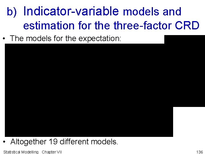
b) Indicator-variable models and estimation for the three-factor CRD • The models for the expectation: • Altogether 19 different models. Statistical Modelling Chapter VII 136
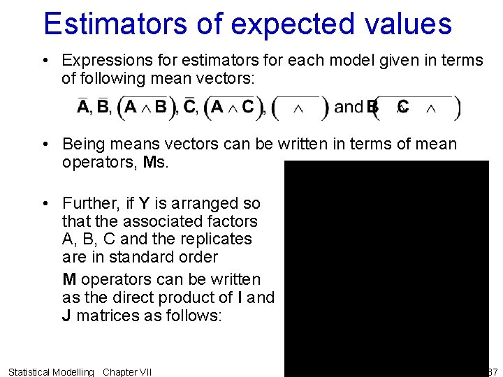
Estimators of expected values • Expressions for estimators for each model given in terms of following mean vectors: • Being means vectors can be written in terms of mean operators, Ms. • Further, if Y is arranged so that the associated factors A, B, C and the replicates are in standard order M operators can be written as the direct product of I and J matrices as follows: Statistical Modelling Chapter VII 137
![c) Expected mean squares under alternative models • Previously given the E[MSq]s under the c) Expected mean squares under alternative models • Previously given the E[MSq]s under the](http://slidetodoc.com/presentation_image_h/004fbee1f5ba79cd59e79fbef1f3d024/image-135.jpg)
c) Expected mean squares under alternative models • Previously given the E[MSq]s under the maximal model. • Also need to consider them under alternative models so that we know what models are indicated by the various hypothesis tests. • Basically, need to know under which models q(y) = 0. • From two-factor case, q(y) = 0 only when the model does not include a term to which the term for the source is marginal. • So, when doing the hypothesis test for a MSq for a fixed term, – provided terms to which it is marginal have been ruled out by prior tests, – it tests whether the expectation term corresponding to it is zero. • For example, consider the A#B mean square. Statistical Modelling Chapter VII 138
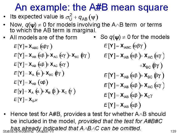
An example: the A#B mean square • Its expected value is • Now, q(y) 0 for models involving the A B term or terms to which the AB term is marginal. • So q(y) 0 for the models • All models are of the form • Hence test for A#B, provides a test for whether A B should be included in the model, provided that the test for A#B#C has already indicated that A B C can be omitted. Statistical Modelling Chapter VII 139
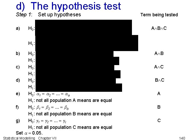
d) The hypothesis test Step 1: a) Set up hypotheses H 0 : Term being tested A B C H 1: b) H 0 : H 1: c) H 0 : H 1: d) H 0 : H 1: e) H 0: a 1 = a 2 =. . . = aa H 1: not all population A means are equal f) H 0: b 1 = b 2 =. . . = bb H 1: not all population B means are equal g) H 0: g 1 = g 2 =. . . = gc H 1: not all population C means are equal Set a = 0. 05. Statistical Modelling Chapter VII A B A C B C A B C 140
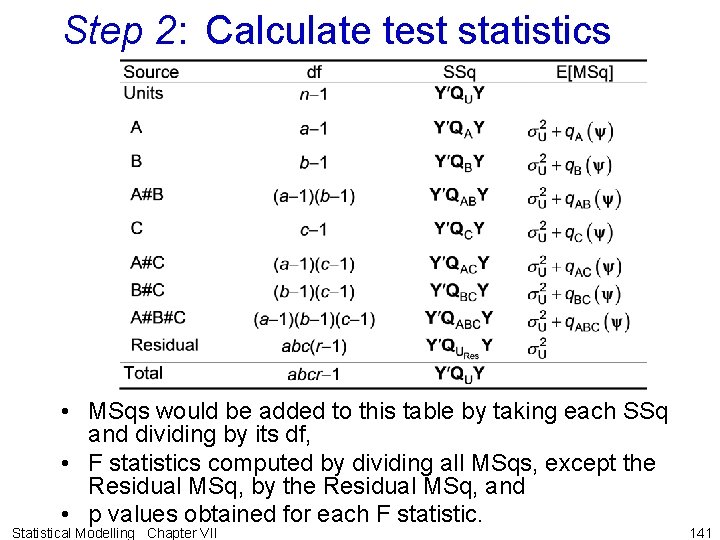
Step 2: Calculate test statistics • MSqs would be added to this table by taking each SSq and dividing by its df, • F statistics computed by dividing all MSqs, except the Residual MSq, by the Residual MSq, and • p values obtained for each F statistic. Statistical Modelling Chapter VII 141
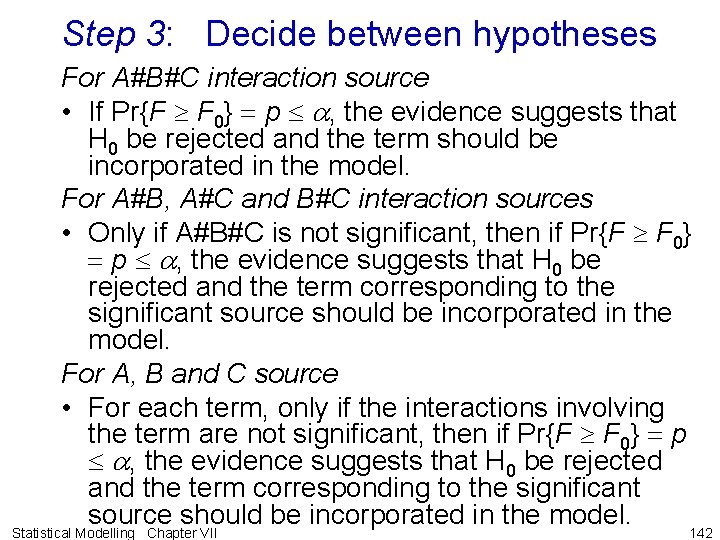
Step 3: Decide between hypotheses For A#B#C interaction source • If Pr{F F 0} = p a, the evidence suggests that H 0 be rejected and the term should be incorporated in the model. For A#B, A#C and B#C interaction sources • Only if A#B#C is not significant, then if Pr{F F 0} = p a, the evidence suggests that H 0 be rejected and the term corresponding to the significant source should be incorporated in the model. For A, B and C source • For each term, only if the interactions involving the term are not significant, then if Pr{F F 0} = p a, the evidence suggests that H 0 be rejected and the term corresponding to the significant source should be incorporated in the model. 142 Statistical Modelling Chapter VII
VII. J Exercises • Ex. VII-1 asks for the complete analysis of a factorial experiment with qualitative factors • Ex. VII-2 involves a nested factorial analysis – not examinable • Ex. VII-3 asks for the complete analysis of a factorial experiment with both factors quantitative • Ex. VII-4 asks for the complete analysis of a factorial experiment with random treatment factors • Ex. VII-5 asks for the complete analysis of a factorial experiment with interactions between unrandomized and randomized factors Statistical Modelling Chapter VII 143
- Slides: 140