Viewing baroclinic initial value problems in terms of

Viewing baroclinic initial value problems in terms of Rossby wave components John Methven, University of Reading Hylke de Vries, University of Reading Tom Frame, University of Reading Brian Hoskins, University of Reading Eyal Heifetz, Tel Aviv University Craig Bishop, Naval Research Laboratories, Monterrey 14 th Cyclone Workshop, 25 September 2008

Motivation Attractive to break down complex flow into a number of components with predictable evolution. Examples 1. Wave-mean flow partition 2. Distinct coherent vortices 3. Wave-like disturbances focussed at different levels Can anticipate what would have happened if basic state or initial disturbances had been different (from physical arguments alone).

Obstacles 1. Appropriate definition of background state 2. Theory for Rossby wave evolution - isolation of Rossby wave components - non-modal growth - nonlinear wave breaking 3. Moisture and latent heat release

Rossby wave components … are waves in potential vorticity (PV). On zonal basic state flows they are advected but also propagate relative to the flow if there is a meridional PV gradient. Linear baroclinic instability interaction between two counterpropagating Rossby waves (CRWs). BUT, the CRW components only describe the evolution of normal modes (the discrete spectrum) [Heifetz et al, 2004]. Is a compact description of evolution possible from general initial conditions (including the continuous spectrum) ? … first consider instability in terms of CRW structures…

Interacting Rossby edge waves When basic state PV is piecewise uniform with only 2 jumps Rayleigh Model Horizontal shear, no vertical variation barotropic instability Eady Model Vertical shear in thermal wind balance with cross-stream temperature gradient and no cross-stream variation in flow baroclinic instability U= z

CRW propagation and interaction

Basic States with Continuous PV Gradients How can a pair of interacting CRWs be identified? n n n Superposing any growing normal mode (NM) and its decaying complex conjugate results an untilted PV structure. Cross-stream wind (v) induced by such PV will also be untilted, as in CRW schematic. Seek 2 CRWs whose phase and amplitude evolution equations have the same form as those for the Eady (or 2 -layer) models.

e. g. , CRW structures in Charney model N S Upper CRW Contours show meridional wind N = northward S = southward Colour shading shows QGPV Red = +ve Blue = -ve S S + + N N Lower CRW +/- indicate boundary temperature anomalies Growing NM in Charney model L=1/k=1000 km

Determining CRW structures from NM PV anomalies of adiabatic NMs arise by meridional displacements of air, η, advecting PV: CRWs are defined as orthogonal in pseudomomentum and “shear term” appearing in pseudoenergy: (=0 for i≠j ) where brackets are defined as Given above defs, PV equation yields evolution equations for CRW amplitudes, a 1, a 2, and phases, ε 1, ε 2, as given by Davies and Bishop (1994) for Eady model. BUT only covers discrete spectrum. What about other PV?

Eady model Initial PV dipole • Uniform vertical shear and static stability • f-plane (no interior PV gradient) • Rigid lid

Eady model Initial PV dipole • Uniform vertical shear and static stability • f-plane (no interior PV gradient) • Rigid lid Black/red = +ve boundary PV anomaly White = -ve boundary PV anomaly

Eady model Initial PV dipole Result at T=12 • Uniform vertical shear and static stability • f-plane (no interior PV gradient) • Rigid lid Red = +ve boundary PV anomaly White = -ve boundary PV anomaly

β-plane with broad tropopause (and no lid)

β-plane with broad tropopause (and no lid)

β-plane with broad tropopause (and no lid) residual PV project

β-plane with broad tropopause (and no lid)

Why is the residual PV almost passive? Consider partitioning PV anomalies: where Substituting into linearised PV equation gives: (1) Meridional wind and parcel displacements are related: Left side of (1) is 0 qp advected as if passive. residual is passive if CRWs describe all of qd for all t

PAR PV approximation Passively advected residual PV approximation “Residual PV” = PV left after subtracting projection onto CRWs. Approximation is that residual evolves by passive advection only. Not exact because residual contains part of qd as well as qp. BUT, partition of q(0) into qd and qp is arbitrary! However, if qp(0)=q(0), qd (0)=0 is assumed, found maximum perturbation energy error (for any t ) < 10%. Can be reduced further by varying initial partition.

Solution to initial value problem under PAR PV approximation 1. 2. 1. 2. Partition q(0) into qd and qp. Project qd onto CRW structures: a 1, a 2, ε 1, ε 2 at t=0 Evolution of qp known qp structure excites CRWs by advection as “forcing” term: j=aj exp(iεj) Amplitude and phase Creation of displacement PV anomalies by winds induced by passive PV

Limitations in application to atmosphere Only 3 Rossby wave components to consider, but… • Theory assumes small amplitude waves (single k) • Partition of large amplitude waves from “background Analysis of state” affects interpretation of evolution nonlinear life cycles Diabatic processes: • 1. Create PV anomalies qp (but need to know history) 2. Latent heat release alters dynamics 3. (e. g. , saturated ascent with reduced effective N 2) • CRW evolution in moist 2 -layer model with ascent/descent asymmetry. • Multi-layer models (but sinusoidal waves).

Bringing Theory and Observation Closer Eady model Simple basic state General jet: U(y, z), Qy(y, z) Sinusoidal wave Unstable NMs Small waveslope QG dynamics CRW pair Dry moisture PE dynamics near balance General initial value problems Continuous spectrum RWs on vertical heating gradients Asymmetry of ascent/descent Large amplitude, but simplified situation Nonlinear life cycle expts Wave-mean interaction Atmosphere RW breaking Stationary waves Simultaneous systems in different stormtracks Water phases

Upper level precursor

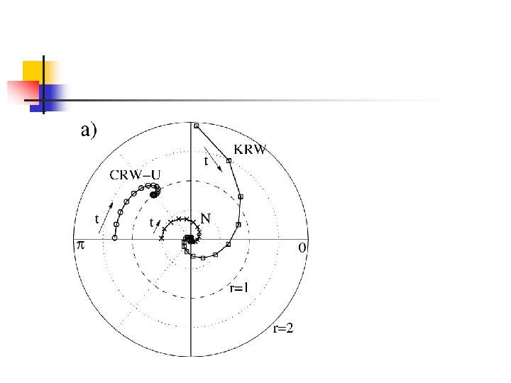
Relative evolution of the CRW components π/2 Angle = U-L phase r ~ tan-1(U/L) Eady t=0 π t=0 0 Charney (+β, no lid) -π/2 Green (+β) π t=0 -π/2 π/2 0 π t=0 -π/2 Broad tropopause 0 (+β, no lid)

β-plane without lid (Charney model)

β-plane + rigid lid (Green model)

β-plane + rigid lid (Green model)