VERY DEEP CONVOLUTIONAL NETWORKS FOR LARGESCALE IMAGE RECOGNITION

VERY DEEP CONVOLUTIONAL NETWORKS FOR LARGE-SCALE IMAGE RECOGNITION does size matter? Karen Simonyan Andrew Zisserman

Contents • • Why I Care Introduction Convolutional Configuration Classification Experiments Conclusion Big Picture

Why I care • 2 nd place in ILSVRC 2014 top-5 val. Challenge

Why I care • 2 nd place in ILSVRC 2014 top-5 val. Challenge • 1 st place in ILSVRC 2014 top-1 val. Challenge

Why I care • 2 nd place in ILSVRC 2014 top-5 val. Challenge • 1 st place in ILSVRC 2014 top-1 val. Challenge • 1 st place in ILSVRC 2014 Localization Challenge

Why I care • • 2 nd place in ILSVRC 2014 top-5 val. Challenge 1 st place in ILSVRC 2014 top-1 val. Challenge 1 st place in ILSVRC 2014 Localization Challenge Demonstrates architecture that works well on diverse datasets

Why I care 2 nd place in ILSVRC 2014 top-5 val. Challenge 1 st place in ILSVRC 2014 top-1 val. Challenge 1 st place in ILSVRC 2014 Localization Challenge Demonstrates architecture that works well on diverse datasets • Demonstrates efficient and effective localization and multi-scaling • •

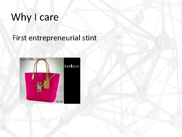
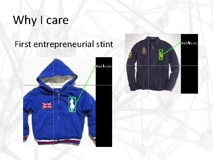
Why I care First entrepreneurial stint

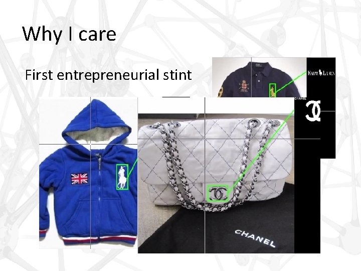
Why I care First entrepreneurial stint

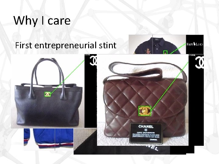
Why I care First entrepreneurial stint

Why I care First entrepreneurial stint

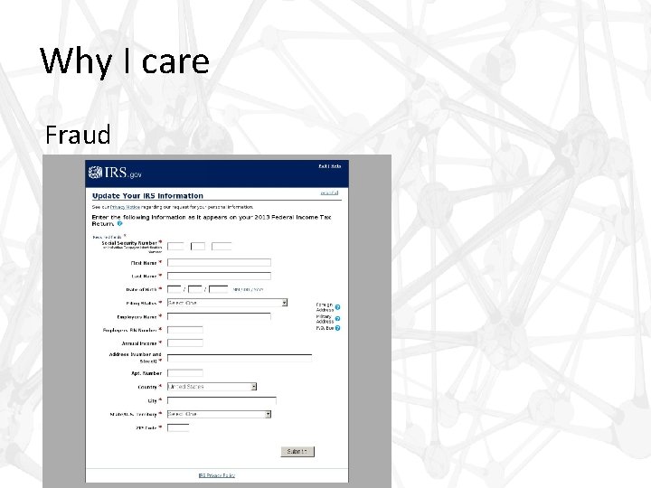
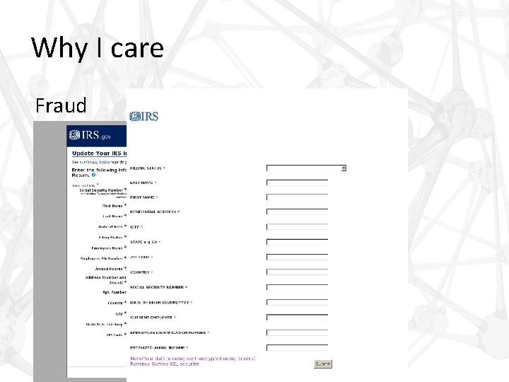
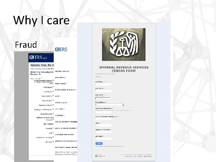
Why I care Fraud

Why I care Fraud

Why I care Fraud

Why I care Fraud

Why I care Fraud

Why I care Fraud

Why I care Fraud

Why I care Fraud

Why I care Fraud

Introduction • Golden age for CNN’s – Krizhevsky et al. 2012 • Establishes new standard

Introduction • Golden age for CNN’s – Krizhevsky et al. 2012 • Establishes new standard – Sermanet et al. 2014 • ‘dense’ application of networks at multiple scales

Introduction • Golden age for CNN’s – Krizhevsky et al. 2012 • Establishes new standard – Sermanet et al. 2014 • ‘dense’ application of networks at multiple scales – Szegedy et al. 2014 • Mixes depth with concatenated inceptions and new topologies

Introduction • Golden age for CNN’s – Krizhevsky et al. 2012 • Establishes new standard – Sermanet et al. 2014 • ‘dense’ application of networks at multiple scales – Szegedy et al. 2014 • Mixes depth with concatenated inceptions and new topologies – Zeiler & Fergus, 2013 – Howard, 2014

Introduction • Key Contributions of Simonyan et al – Systematic evaluation of depth of CNN architecture • Steadily increase the depth of the network by adding more convolutional layers, while holding other parameters fixed • Use very small (3 × 3) convolution filters in all layers

Introduction • Key Contributions of Simonyan et al – Systematic evaluation of depth of CNN architecture – Achieves state of the art accuracy in ILSVRC classification and localization • • 2 nd place in ILSVRC 2014 top-5 val. Challenge 1 st place in ILSVRC 2014 top-1 val. Challenge 1 st place in ILSVRC 2014 Localization Challenge Demonstrates architecture that works well on diverse datasets

Introduction • Key Contributions of Simonyan et al – Systematic evaluation of depth of CNN architecture – Achieves state of the art accuracy in ILSVRC classification and localization – Achieves state of the art in Caltech and VOC datasets

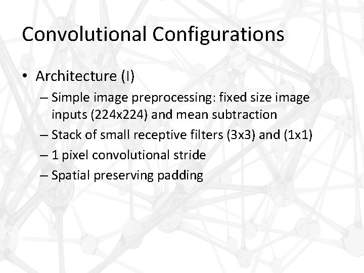
Convolutional Configurations • Architecture (I) – Simple image preprocessing: fixed size image inputs (224 x 224) and mean subtraction

Convolutional Configurations • Architecture (I) – Simple image preprocessing: fixed size image inputs (224 x 224) and mean subtraction – Stack of small receptive filters (3 x 3) and (1 x 1)

Convolutional Configurations • Architecture (I) – Simple image preprocessing: fixed size image inputs (224 x 224) and mean subtraction – Stack of small receptive filters (3 x 3) and (1 x 1) – 1 pixel convolutional stride

Convolutional Configurations • Architecture (I) – Simple image preprocessing: fixed size image inputs (224 x 224) and mean subtraction – Stack of small receptive filters (3 x 3) and (1 x 1) – 1 pixel convolutional stride – Spatial preserving padding

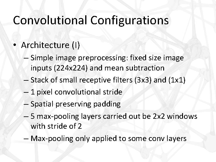
Convolutional Configurations • Architecture (I) – Simple image preprocessing: fixed size image inputs (224 x 224) and mean subtraction – Stack of small receptive filters (3 x 3) and (1 x 1) – 1 pixel convolutional stride – Spatial preserving padding – 5 max-pooling layers carried out be 2 x 2 windows with stride of 2

Convolutional Configurations • Architecture (I) – Simple image preprocessing: fixed size image inputs (224 x 224) and mean subtraction – Stack of small receptive filters (3 x 3) and (1 x 1) – 1 pixel convolutional stride – Spatial preserving padding – 5 max-pooling layers carried out be 2 x 2 windows with stride of 2 – Max-pooling only applied to some conv layers

Convolutional Configurations • Architecture (II) – A variable stack of Convolutional layers (parameterized by depth)

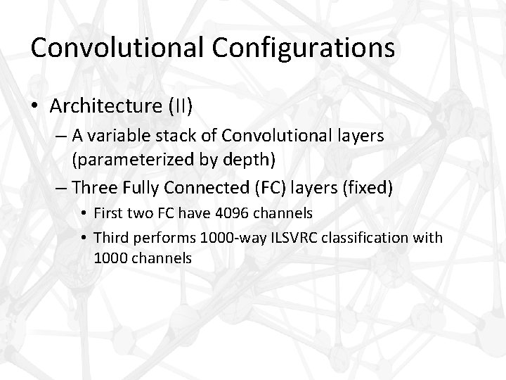
Convolutional Configurations • Architecture (II) – A variable stack of Convolutional layers (parameterized by depth) – Three Fully Connected (FC) layers (fixed) • First two FC have 4096 channels • Third performs 1000 -way ILSVRC classification with 1000 channels

Convolutional Configurations • Architecture (II) – A variable stack of Convolutional layers (parameterized by depth) – Three Fully Connected (FC) layers (fixed) • First two FC have 4096 channels • Third performs 1000 -way ILSVRC classification with 1000 channels – Hidden layers use Re. LU non-linearity

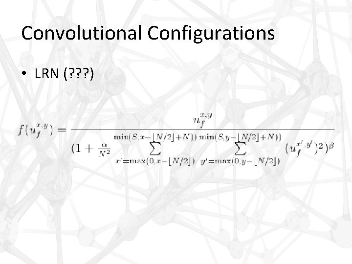
Convolutional Configurations • Architecture (II) – A variable stack of Convolutional layers (parameterized by depth) – Three Fully Connected (FC) layers (fixed) • First two FC have 4096 channels • Third performs 1000 -way ILSVRC classification with 1000 channels – Hidden layers use Re. LU non-linearity – Also test Local Response Normalization (LRN) ? ? ?

Convolutional Configurations • LRN (? ? ? )

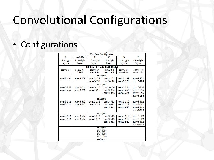
Convolutional Configurations • Configurations – 11 to 19 weight layers

Convolutional Configurations • Configurations – 11 to 19 weight layers – Convolutional layer width increases by factor of 2 after each max-pooling; eg, 64, 128, 512 etc

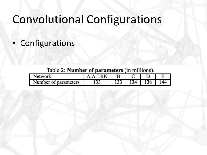
Convolutional Configurations • Configurations – 11 to 19 weight layers – Convolutional layer width increases by factor of 2 after each max-pooling; eg, 64, 128, 512 etc – Key observation: although depth increases, total parameters are loosely conserved compared to shallower CNN’s with larger receptive fields (example all tested nets <= 144 M (Sermanet))

Convolutional Configurations • Configurations

Convolutional Configurations • Configurations

Convolutional Configurations • Remarks – Configurations use stacks of small filters (3 x 3) and (1 x 1) with 1 pixel strides

Convolutional Configurations • Remarks – Configurations use stacks of small filters (3 x 3) and (1 x 1) with 1 pixel strides – drastic change from larger receptive fields and strides • Eg. 11× 11 with stride 4 in (Krizhevsky et al. , 2012) • Eg. 7× 7 with stride 2 in (Zeiler & Fergus, 2013; Sermanet et al. , 2014))

Convolutional Configurations • Remarks – Decreases parameters with same effective receptive field • Consider triple stack of (3 x 3) filters and a single (7 x 7) filter • The two have same effective receptive field (7 x 7) • Single (7 x 7) has parameters proportional to 49 • Triple (3 x 3) stack has parameters proportional to 3 x(3 x 3) = 27

Convolutional Configurations • Remarks – Decreases parameters with same effective receptive field – Additional conv. Layers add non-linearities introduced by the rectification function

Convolutional Configurations • Remarks – Decreases parameters with same effective receptive field – Additional conv. Layers add non-linearities introduced by the rectification function – Small conv filters also used by Ciresan et al. (2012), and Goog. Le. Net (Szegedy et al. , 2014)

Convolutional Configurations • Remarks – Decreases parameters with same effective receptive field – Additional conv. Layers add non-linearities introduced by the rectification function – Small conv filters also used by Ciresan et al. (2012), and Goog. Le. Net (Szegedy et al. , 2014) – Szegedy also uses VERY deep net (22 weight layers) with complex topology for Goog. Le. Net

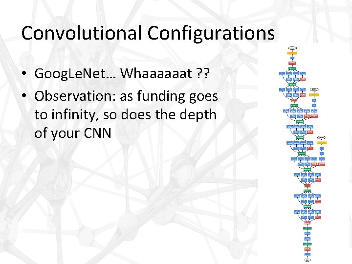
Convolutional Configurations • Goog. Le. Net… Whaaaaaat ? ? • Observation: as funding goes to infinity, so does the depth of your CNN

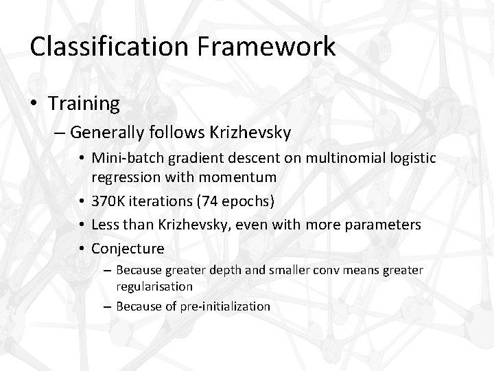
Classification Framework • Training – Generally follows Krizhevsky • Mini-batch gradient descent on multinomial logistic regression with momentum – – Batch size: 256 Momentum: 0. 9 Weight decay: 5 x 10 -4 Drop out ratio: 0. 5

Classification Framework • Training – Generally follows Krizhevsky • Mini-batch gradient descent on multinomial logistic regression with momentum • 370 K iterations (74 epochs) • Less than Krizhevsky, even with more parameters • Conjecture – Because greater depth and smaller conv means greater regularisation – Because of pre-initialization

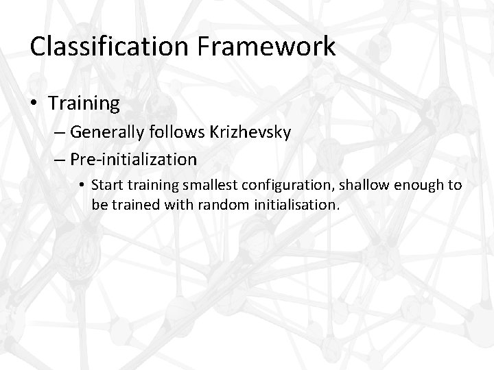
Classification Framework • Training – Generally follows Krizhevsky – Pre-initialization • Start training smallest configuration, shallow enough to be trained with random initialisation.

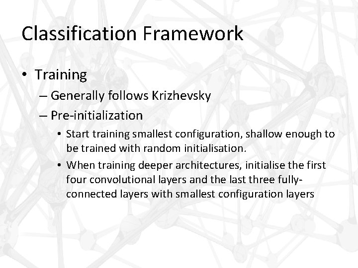
Classification Framework • Training – Generally follows Krizhevsky – Pre-initialization • Start training smallest configuration, shallow enough to be trained with random initialisation. • When training deeper architectures, initialise the first four convolutional layers and the last three fullyconnected layers with smallest configuration layers

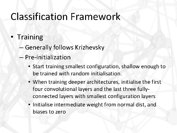
Classification Framework • Training – Generally follows Krizhevsky – Pre-initialization • Start training smallest configuration, shallow enough to be trained with random initialisation. • When training deeper architectures, initialise the first four convolutional layers and the last three fullyconnected layers with smallest configuration layers • Initialise intermediate weight from normal dist, and biases to zero

Classification Framework • Training – Generally follows Krizhevsky – Pre-initialization – Augmentation and cropping • Each batch, each image is randomly cropped to fit fixed 224 x 224 input

Classification Framework • Training – Generally follows Krizhevsky – Pre-initialization – Augmentation and cropping • Each batch, each image is randomly cropped to fit fixed 224 x 224 input • Augmentation via random horizontal flipping and random RGB color shift

Classification Framework • Training – Generally follows Krizhevsky – Pre-initialization – Augmentation and cropping – Training image size • Let S be smallest size of isotropically rescaled image, such that S >= 224

Classification Framework • Training – Generally follows Krizhevsky – Pre-initialization – Augmentation and cropping – Training image size • Let S be smallest size of isotropically rescaled image, such that S >= 224 • Approach 1: fixed scale; try both S = 256 and 384

Classification Framework • Training – Generally follows Krizhevsky – Pre-initialization – Augmentation and cropping – Training image size • Let S be smallest size of isotropically rescaled image, such that S >= 224 • Approach 1: fixed scale; try both S = 256 and 384 • Approach 2: multi-scale training; randomly resample from certain range [256, 512]

Classification Framework • Testing – Network is applied ‘densely’ to whole image, inspired by Sermanet et al 2014 • Image is rescaled to Q (not necessarily = S)

Classification Framework • Testing – Network is applied ‘densely’ to whole image, inspired by Sermanet et al 2014 • Image is rescaled to Q (not necessarily = S) • The final fully connected layers are converted to convolutional layers (? ? ? )

Classification Framework • Testing – Network is applied ‘densely’ to whole image, inspired by Sermanet et al 2014 • Image is rescaled to Q (not necessarily = S) • The final fully connected layers are converted to convolutional layers (? ? ? ) • The resulting fully convolutional net is then applied to whole image, without need for cropping

Classification Framework • Testing – Network is applied ‘densely’ to whole image, inspired by Sermanet et al 2014 • Image is rescaled to Q (not necessarily = S) • The final fully connected layers are converted to convolutional layers (? ? ? ) • The resulting fully convolutional net is then applied to whole image, without need for cropping • Spatial output map is spatially averaged to get fixed vector output

Classification Framework • Testing – Network is applied ‘densely’ to whole image, inspired by Sermanet et al 2014 • Image is rescaled to Q (not necessarily = S) • The final fully connected layers are converted to convolutional layers (? ? ? ) • The resulting fully convolutional net is then applied to whole image, without need for cropping • Spatial output map is spatially averaged to get fixed vector output • Augment test set by horizontal flipping

Classification Framework • Testing – Network is applied ‘densely’ to whole image – Remarks • Dense application works on whole image

Classification Framework • Testing – Network is applied ‘densely’ to whole image – Remarks • Dense application works on whole image • Krizhevsky 2012 and Szegedy 2014 uses multiple crops at test time

Classification Framework • Testing – Network is applied ‘densely’ to whole image – Remarks • Dense application works on whole image • Krizhevsky 2012 and Szegedy 2014 uses multiple crops at test time • Two approaches have accuracy-time tradeoff

Classification Framework • Testing – Network is applied ‘densely’ to whole image – Remarks • Dense application works on whole image • Krizhevsky 2012 and Szegedy 2014 uses multiple crops at test time • Two approaches have accuracy-time tradeoff • They can be implemented complementarily; only change is that features have different padding

Classification Framework • Testing – Network is applied ‘densely’ to whole image – Remarks • Dense application works on whole image • Krizhevsky 2012 and Szegedy 2014 uses multiple crops at test time • Two approaches have accuracy-time tradeoff • They can be implemented complementarily; only change is that features have different padding • Also test using 50 crops /scale

Classification Framework • Implementation – Derived from public C++ Caffe toolbox (Jia, 2013) – Modified to train and evaluate on multiple GPU’s – Designed for uncropped images at multiple scales – Optimized around batch parallelism – Synchoronous gradient computation – 3. 75 x speedup compared to single GPU – 2 -3 weeks training

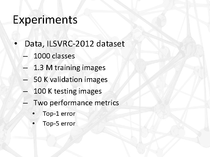
Experiments • Data, ILSVRC-2012 dataset – – – 1000 classes 1. 3 M training images 50 K validation images 100 K testing images Two performance metrics • • Top-1 error Top-5 error

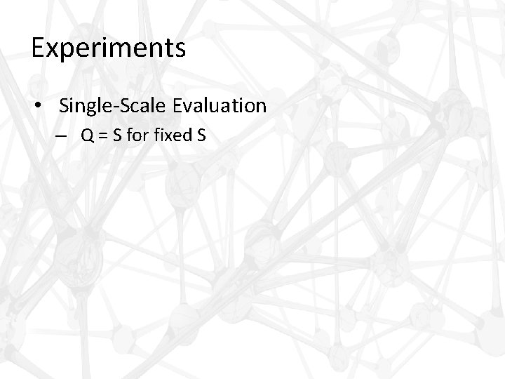
Experiments • Single-Scale Evaluation – Q = S for fixed S

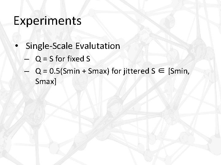
Experiments • Single-Scale Evalutation – Q = S for fixed S – Q = 0. 5(Smin + Smax) for jittered S ∈ [Smin, Smax]

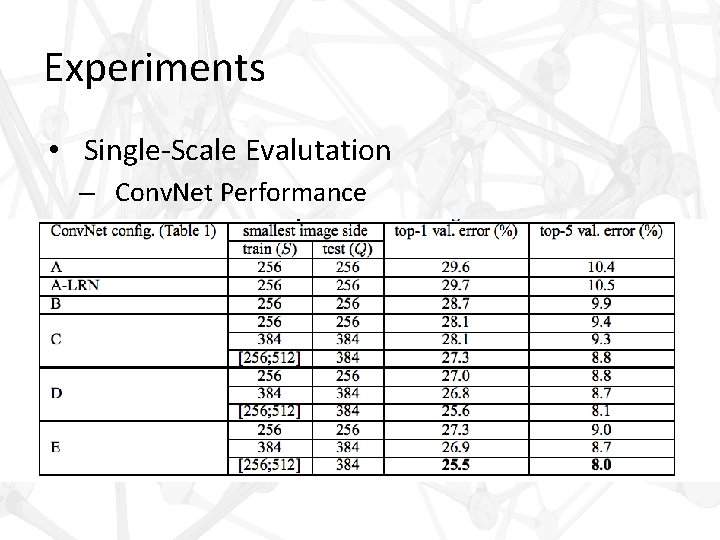
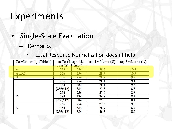
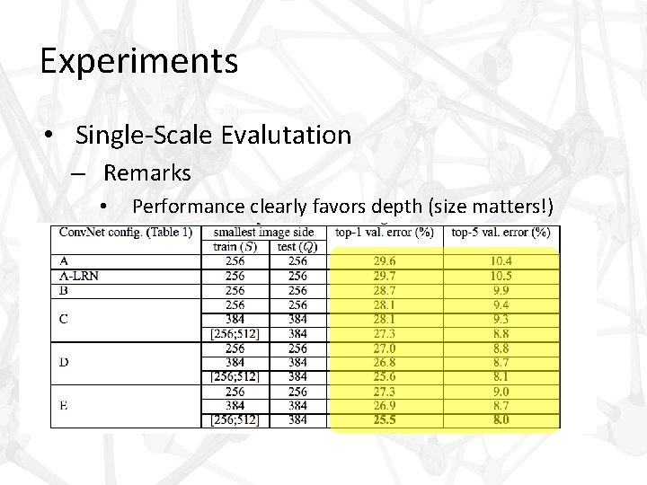
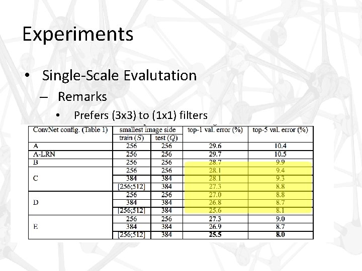
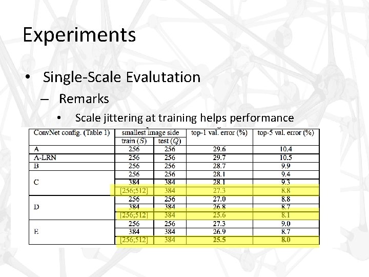
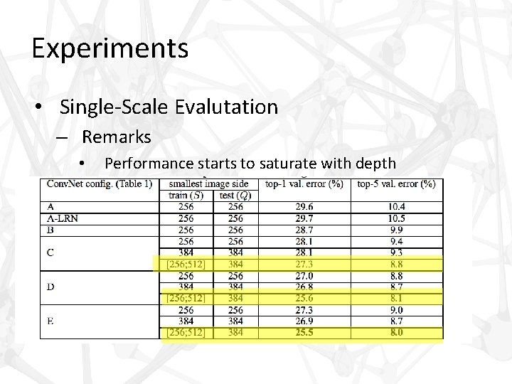
Experiments • Single-Scale Evalutation – Conv. Net Performance

Experiments • Single-Scale Evalutation – Remarks • Local Response Normalization doesn’t help

Experiments • Single-Scale Evalutation – Remarks • Performance clearly favors depth (size matters!)

Experiments • Single-Scale Evalutation – Remarks • Prefers (3 x 3) to (1 x 1) filters

Experiments • Single-Scale Evalutation – Remarks • Scale jittering at training helps performance

Experiments • Single-Scale Evalutation – Remarks • Performance starts to saturate with depth

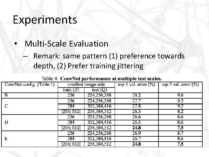
Experiments • Multi-Scale Evaluation – Run model over several rescaled versions, or Q-values, and average resulting posteriors

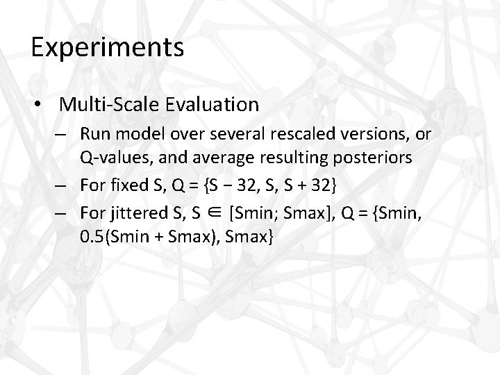
Experiments • Multi-Scale Evaluation – Run model over several rescaled versions, or Q-values, and average resulting posteriors – For fixed S, Q = {S − 32, S, S + 32}

Experiments • Multi-Scale Evaluation – Run model over several rescaled versions, or Q-values, and average resulting posteriors – For fixed S, Q = {S − 32, S, S + 32} – For jittered S, S ∈ [Smin; Smax], Q = {Smin, 0. 5(Smin + Smax), Smax}

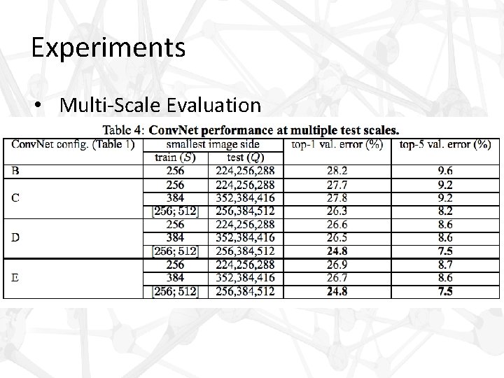
Experiments • Multi-Scale Evaluation

Experiments • Multi-Scale Evaluation – Remark: same pattern (1) preference towards depth, (2) Prefer training jittering

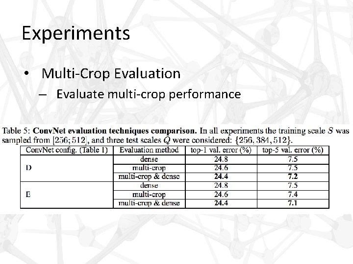
Experiments • Multi-Crop Evaluation – Evaluate multi-crop performance

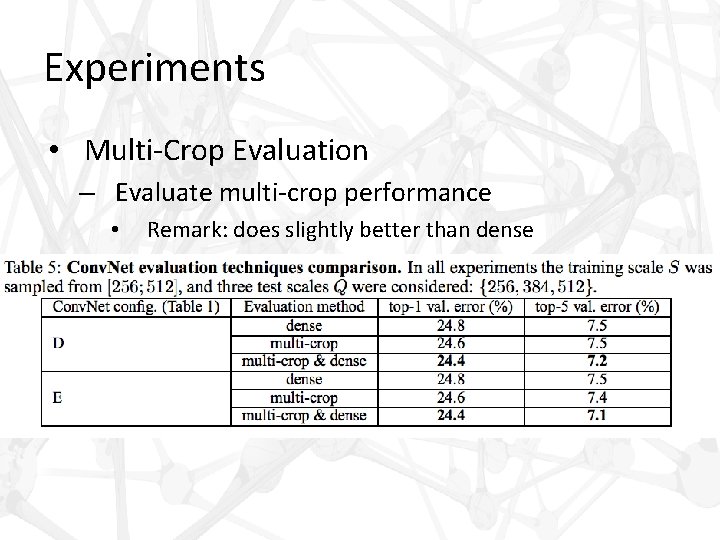
Experiments • Multi-Crop Evaluation – Evaluate multi-crop performance • Remark: does slightly better than dense

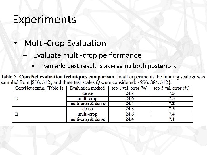
Experiments • Multi-Crop Evaluation – Evaluate multi-crop performance • Remark: best result is averaging both posteriors

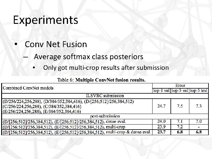
Experiments • Conv Net Fusion – Average softmax class posteriors • Only got multi-crop results after submission

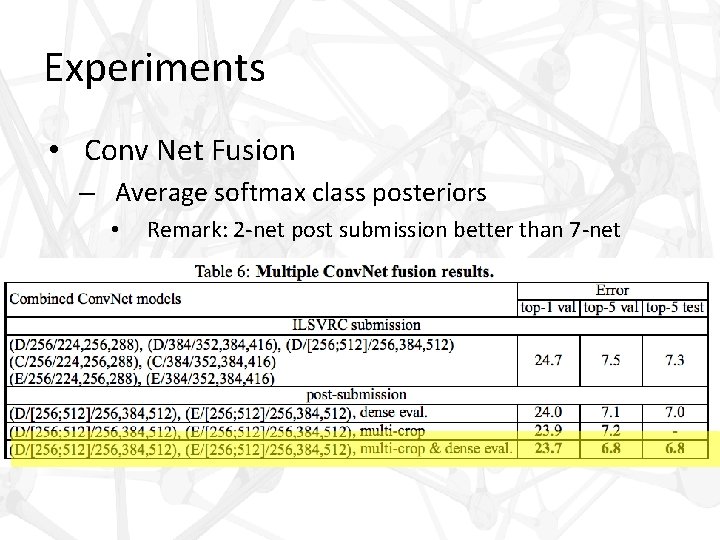
Experiments • Conv Net Fusion – Average softmax class posteriors • Remark: 2 -net post submission better than 7 -net

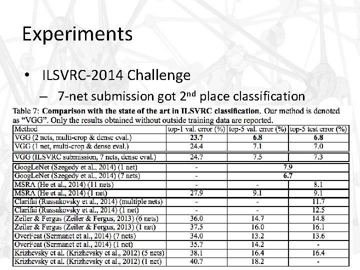
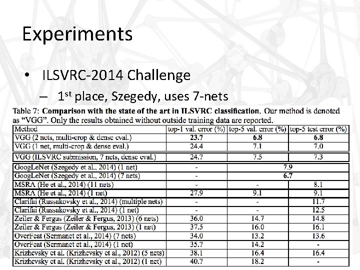
Experiments • ILSVRC-2014 Challenge – 7 -net submission got 2 nd place classification

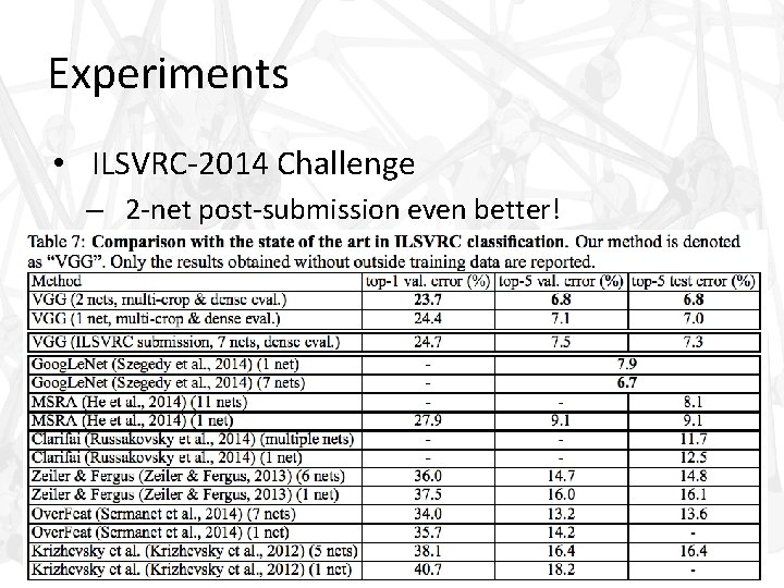
Experiments • ILSVRC-2014 Challenge – 2 -net post-submission even better!

Experiments • ILSVRC-2014 Challenge – 1 st place, Szegedy, uses 7 -nets

Localization • Inspired by Sermanet et al – Special case of object detection

Localization • Inspired by Sermanet et al – Special case of object detection – Predicts single object bounding box for each of the top-5 classes, irrespective of the actual number of objects of the class

Localization • Method – Architecture • Same very deep architecture (D) • Includes 4 -D bounding box prediction

Localization • Method – Architecture • Same very deep architecture (D) • Includes 4 -D bounding box prediction • Two cases – Single-class regression (SCR); last layer is 4 -D – Per-class regression (PCR); last layer is 4000 -D

Localization • Method – Architecture – Training • Replace logistic regression objective with Euclidean loss based on bounding box prediction from ground truth

Localization • Method – Architecture – Training • Replace logistic regression objective with Euclidean loss based on bounding box prediction from ground truth • Only trained on fixed size S = 256 and 384

Localization • Method – Architecture – Training • Replace logistic regression objective with Euclidean loss based on bounding box prediction from ground truth • Only trained on fixed size S = 256 and 384 • Initialized the same way as classification model

Localization • Method – Architecture – Training • Replace logistic regression objective with Euclidean loss based on bounding box prediction from ground truth • Only trained on fixed size S = 256 and 384 • Initialized the same way as classification model • Tried fine-tuning (? ? ? ) all layers and only first 2 FC layers

Localization • Method – Architecture – Training • Replace logistic regression objective with Euclidean loss based on bounding box prediction from ground truth • Only trained on fixed size S = 256 and 384 • Initialized the same way as classification model • Tried fine-tuning (? ? ? ) all layers and only first 2 FC layers • Last FC layer was initialized and trained from scratch

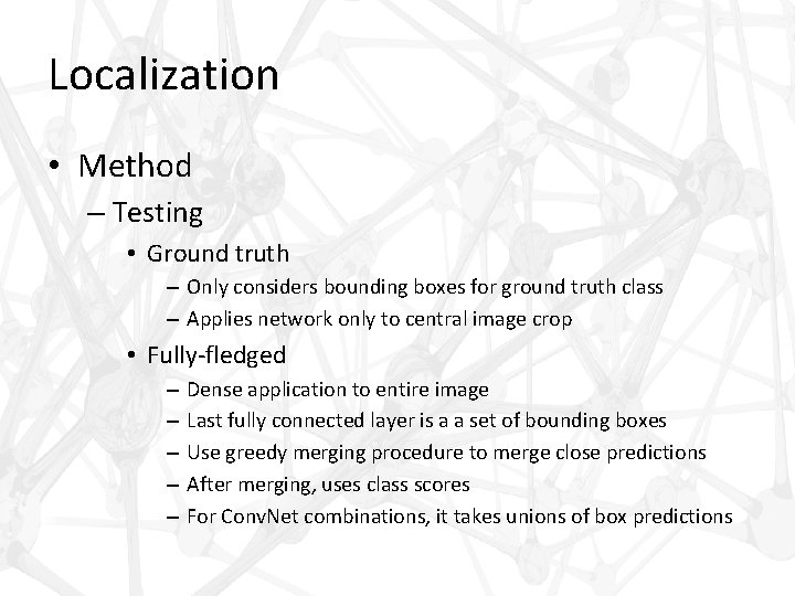
Localization • Method – Testing • Ground truth – Only considers bounding boxes for ground truth class

Localization • Method – Testing • Ground truth – Only considers bounding boxes for ground truth class – Applies network only to central image crop

Localization • Method – Testing • Ground truth – Only considers bounding boxes for ground truth class – Applies network only to central image crop • Fully-fledged – Dense application to entire image

Localization • Method – Testing • Ground truth – Only considers bounding boxes for ground truth class – Applies network only to central image crop • Fully-fledged – Dense application to entire image – Last fully connected layer is a a set of bounding boxes

Localization • Method – Testing • Ground truth – Only considers bounding boxes for ground truth class – Applies network only to central image crop • Fully-fledged – Dense application to entire image – Last fully connected layer is a a set of bounding boxes – Use greedy merging procedure to merge close predictions

Localization • Method – Testing • Ground truth – Only considers bounding boxes for ground truth class – Applies network only to central image crop • Fully-fledged – – Dense application to entire image Last fully connected layer is a a set of bounding boxes Use greedy merging procedure to merge close predictions After merging, uses class scores

Localization • Method – Testing • Ground truth – Only considers bounding boxes for ground truth class – Applies network only to central image crop • Fully-fledged – – – Dense application to entire image Last fully connected layer is a a set of bounding boxes Use greedy merging procedure to merge close predictions After merging, uses class scores For Conv. Net combinations, it takes unions of box predictions

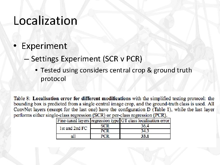
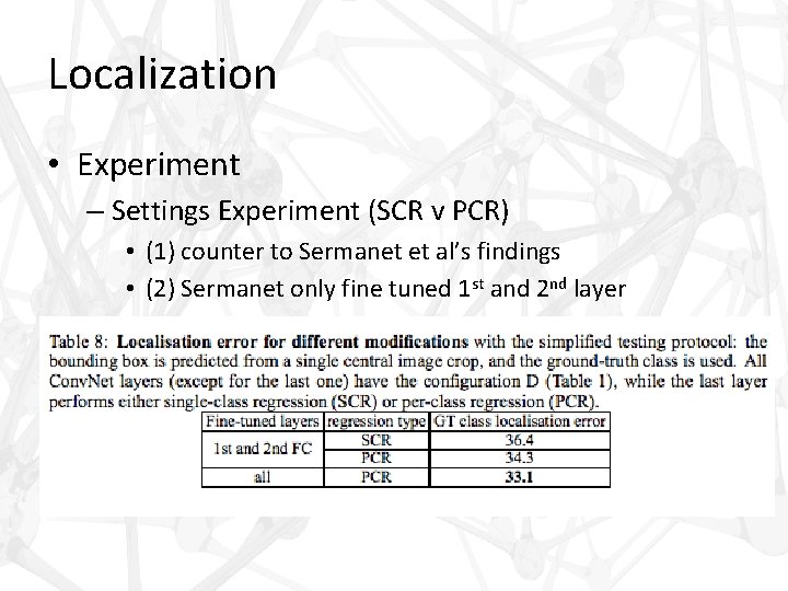
Localization • Experiment – Settings Experiment (SCR v PCR) • Tested using considers central crop & ground truth protocol

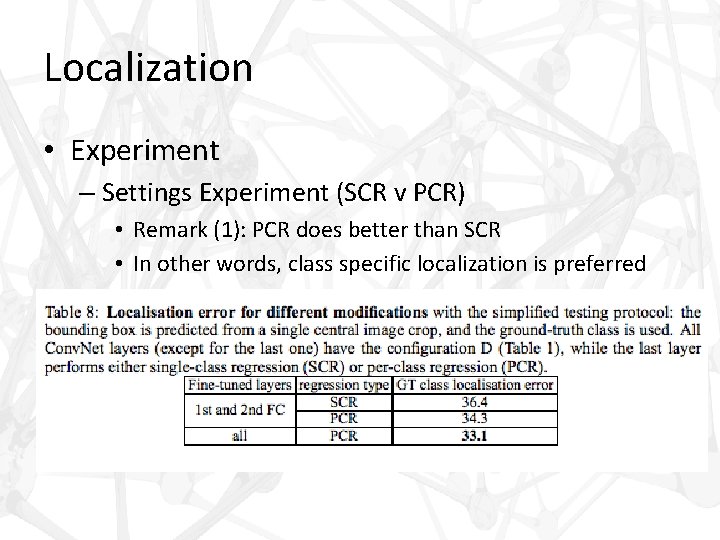
Localization • Experiment – Settings Experiment (SCR v PCR) • Remark (1): PCR does better than SCR • In other words, class specific localization is preferred

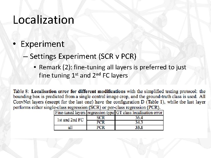
Localization • Experiment – Settings Experiment (SCR v PCR) • Remark (2): fine-tuning all layers is preferred to just fine tuning 1 st and 2 nd FC layers

Localization • Experiment – Settings Experiment (SCR v PCR) • (1) counter to Sermanet et al’s findings • (2) Sermanet only fine tuned 1 st and 2 nd layer

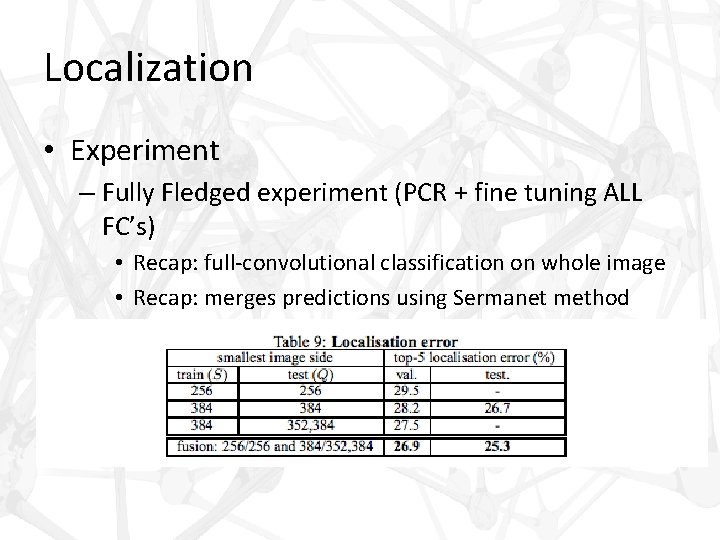
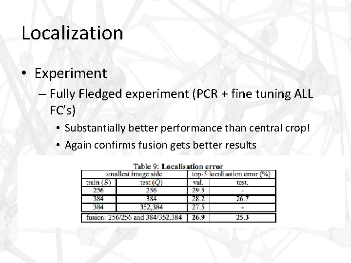
Localization • Experiment – Fully Fledged experiment (PCR + fine tuning ALL FC’s) • Recap: full-convolutional classification on whole image • Recap: merges predictions using Sermanet method

Localization • Experiment – Fully Fledged experiment (PCR + fine tuning ALL FC’s) • Substantially better performance than central crop!

Localization • Experiment – Fully Fledged experiment (PCR + fine tuning ALL FC’s) • Substantially better performance than central crop! • Again confirms fusion gets better results

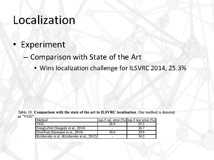
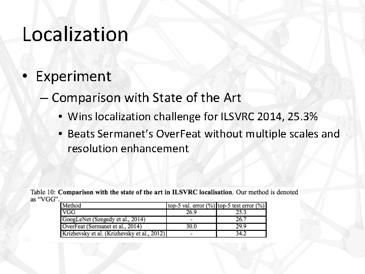
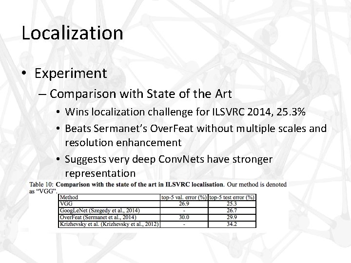
Localization • Experiment – Comparison with State of the Art • Wins localization challenge for ILSVRC 2014, 25. 3%

Localization • Experiment – Comparison with State of the Art • Wins localization challenge for ILSVRC 2014, 25. 3% • Beats Sermanet’s Over. Feat without multiple scales and resolution enhancement

Localization • Experiment – Comparison with State of the Art • Wins localization challenge for ILSVRC 2014, 25. 3% • Beats Sermanet’s Over. Feat without multiple scales and resolution enhancement • Suggests very deep Conv. Nets have stronger representation

Generalization of Very Deep Features • Demand for application on smaller datasets – ILSVRC derived Conv. Net feature extractors have outperformed hand-crafted representations by a large margin

Generalization of Very Deep Features • Demand for application on smaller datasets – ILSVRC derived Conv. Net feature extractors have outperformed hand-crafted representations by a large margin – Approach for smaller datasets • Remove last 1000 -D fully connected layer

Generalization of Very Deep Features • Demand for application on smaller datasets – ILSVRC derived Conv. Net feature extractors have outperformed hand-crafted representations by a large margin – Approach for smaller datasets • Remove last 1000 -D fully connected layer • Use penultimate 4096 -D layer as input to SVM

Generalization of Very Deep Features • Demand for application on smaller datasets – ILSVRC derived Conv. Net feature extractors have outperformed hand-crafted representations by a large margin – Approach for smaller datasets • Remove last 1000 -D fully connected layer • Use penultimate 4096 -D layer as input to SVM • Train SVM on smaller dataset

Generalization of Very Deep Features • Demand for application on smaller datasets – Evaluation is similar to regular dense application • • Rescale to Q apply network densely over whole image Global average pooling on resulting 4096 -D descriptor Horizontal flipping

Generalization of Very Deep Features • Demand for application on smaller datasets – Evaluation is similar to regular dense application • • • Rescale to Q apply network densely over whole image Global average pooling on resulting 4096 -D descriptor Horizontal flipping Pooling over multiple scales – Other approaches stack descriptors of different scales – Results in increasing dimensionality of descriptor

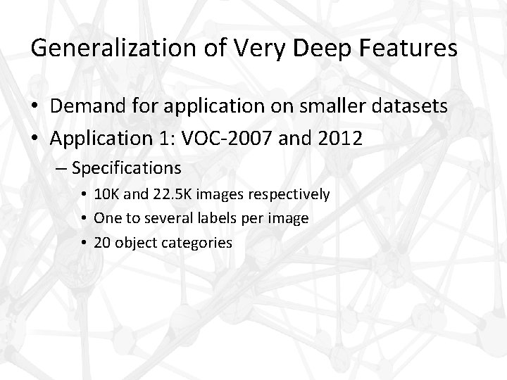
Generalization of Very Deep Features • Demand for application on smaller datasets • Application 1: VOC-2007 and 2012 – Specifications • 10 K and 22. 5 K images respectively • One to several labels per image • 20 object categories

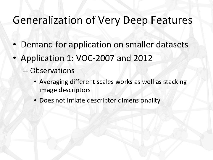
Generalization of Very Deep Features • Demand for application on smaller datasets • Application 1: VOC-2007 and 2012 – Observations • Averaging different scales works as well as stacking image descriptors • Does not inflate descriptor dimensionality

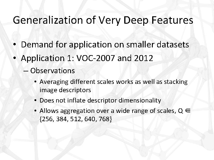
Generalization of Very Deep Features • Demand for application on smaller datasets • Application 1: VOC-2007 and 2012 – Observations • Averaging different scales works as well as stacking image descriptors • Does not inflate descriptor dimensionality • Allows aggregation over a wide range of scales, Q ∈ {256, 384, 512, 640, 768}

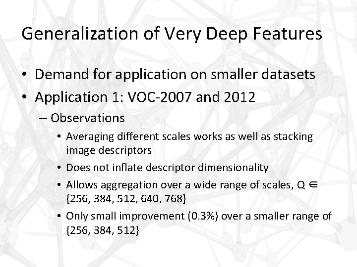
Generalization of Very Deep Features • Demand for application on smaller datasets • Application 1: VOC-2007 and 2012 – Observations • Averaging different scales works as well as stacking image descriptors • Does not inflate descriptor dimensionality • Allows aggregation over a wide range of scales, Q ∈ {256, 384, 512, 640, 768} • Only small improvement (0. 3%) over a smaller range of {256, 384, 512}

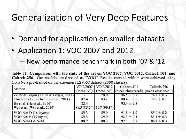
Generalization of Very Deep Features • Demand for application on smaller datasets • Application 1: VOC-2007 and 2012 – New performance benchmark in both ’ 07 & ‘ 12!

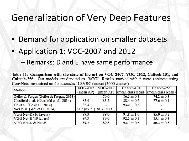
Generalization of Very Deep Features • Demand for application on smaller datasets • Application 1: VOC-2007 and 2012 – Remarks: D and E have same performance

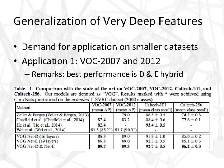
Generalization of Very Deep Features • Demand for application on smaller datasets • Application 1: VOC-2007 and 2012 – Remarks: best performance is D & E hybrid

Generalization of Very Deep Features • Demand for application on smaller datasets • Application 1: VOC-2007 and 2012 – Remarks: Wei et al 2012 result has extra training

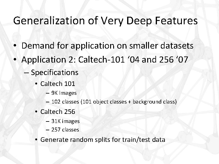
Generalization of Very Deep Features • Demand for application on smaller datasets • Application 2: Caltech-101 ‘ 04 and 256 ‘ 07 – Specifications • Caltech 101 – 9 K Images – 102 classes (101 object classes + background class) • Caltech 256 – 31 K images – 257 classes • Generate random splits for train/test data

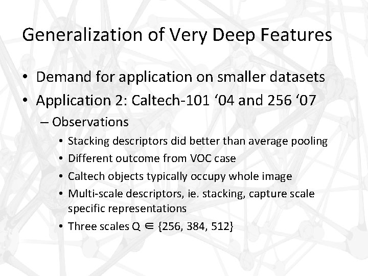
Generalization of Very Deep Features • Demand for application on smaller datasets • Application 2: Caltech-101 ‘ 04 and 256 ‘ 07 – Observations • Stacking descriptors did better than average pooling

Generalization of Very Deep Features • Demand for application on smaller datasets • Application 2: Caltech-101 ‘ 04 and 256 ‘ 07 – Observations • Stacking descriptors did better than average pooling • Different outcome from VOC case

Generalization of Very Deep Features • Demand for application on smaller datasets • Application 2: Caltech-101 ‘ 04 and 256 ‘ 07 – Observations • Stacking descriptors did better than average pooling • Different outcome from VOC case • Caltech objects typically occupy whole image

Generalization of Very Deep Features • Demand for application on smaller datasets • Application 2: Caltech-101 ‘ 04 and 256 ‘ 07 – Observations • • Stacking descriptors did better than average pooling Different outcome from VOC case Caltech objects typically occupy whole image Multi-scale descriptors, ie. stacking, capture scale specific representations

Generalization of Very Deep Features • Demand for application on smaller datasets • Application 2: Caltech-101 ‘ 04 and 256 ‘ 07 – Observations Stacking descriptors did better than average pooling Different outcome from VOC case Caltech objects typically occupy whole image Multi-scale descriptors, ie. stacking, capture scale specific representations • Three scales Q ∈ {256, 384, 512} • •

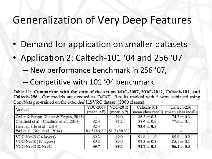
Generalization of Very Deep Features • Demand for application on smaller datasets • Application 2: Caltech-101 ‘ 04 and 256 ‘ 07 – New performance benchmark in 256 ’ 07, – Competitive with 101 ’ 04 benchmark

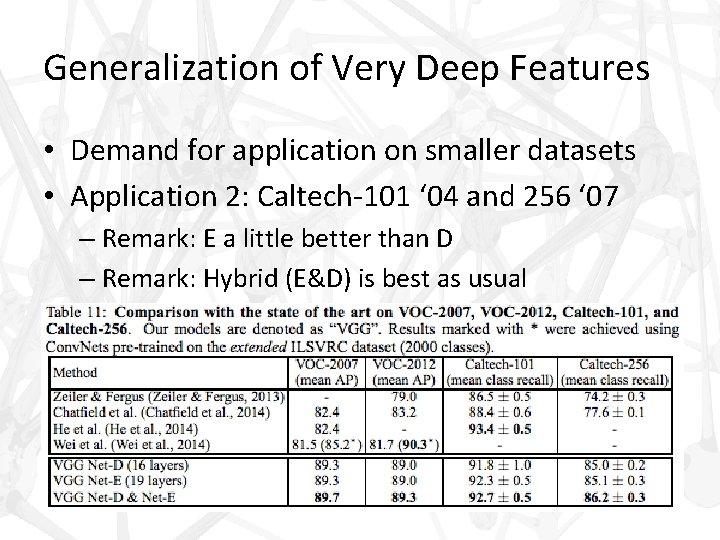
Generalization of Very Deep Features • Demand for application on smaller datasets • Application 2: Caltech-101 ‘ 04 and 256 ‘ 07 – Remark: E a little better than D – Remark: Hybrid (E&D) is best as usual

Generalization of Very Deep Features • Demand for application on smaller datasets • Other Recognition Tasks – Active demand for a wide range of image recognition tasks, consistently outperforming more shallow representations. • Object detection (Girshick et al. 2014)

Generalization of Very Deep Features • Demand for application on smaller datasets • Other Recognition Tasks – Active demand for a wide range of image recognition tasks, consistently outperforming more shallow representations. • Object detection (Girshick et al. 2014) • Semantic segmentation (Long et al. , 2014),

Generalization of Very Deep Features • Demand for application on smaller datasets • Other Recognition Tasks – Active demand for a wide range of image recognition tasks, consistently outperforming more shallow representations. • Object detection (Girshick et al. 2014) • Semantic segmentation (Long et al. , 2014), • Image caption generation (Kiros et al. , 2014; Karpathy & Fei-Fei, 2014)

Generalization of Very Deep Features • Demand for application on smaller datasets • Other Recognition Tasks – Active demand for a wide range of image recognition tasks, consistently outperforming more shallow representations. • Object detection (Girshick et al. 2014) • Semantic segmentation (Long et al. , 2014), • Image caption generation (Kiros et al. , 2014; Karpathy & Fei-Fei, 2014) • Texture and material recognition (Cimpoi et al. , 2014; Bell et al. , 2014).

Conclusion • Demonstrated depth increase benefits performance accuracy (size matters!)

Conclusion • Demonstrated depth increase benefits performance accuracy (size matters!) • Achieves 2 nd place in ILSVRC 2014 Challenge – Achieves 2 nd place in top-5 val error (7. 5%) – Achieves 1 st place in top-1 val error (24. 7%)

Conclusion • Demonstrated depth increase benefits performance accuracy (size matters!) • Achieves 2 nd place in ILSVRC 2014 Challenge – Achieves 2 nd place in top-5 val error (7. 5%) – Achieves 1 st place in top-1 val error (24. 7%) – 7. 0% & 11. 2% better than prior winners

Conclusion • Demonstrated depth increase benefits performance accuracy (size matters!) • Achieves 2 nd place in ILSVRC 2014 Challenge – Achieves 2 nd place in top-5 val error (7. 5%) – Achieves 1 st place in top-1 val error (24. 7%) – 7. 0% & 11. 2% better than prior winners – Post submission got 6. 8% with only 2 -nets – Szegedy got 1 st 6. 7% with 7 -nets

Conclusion • Demonstrated depth increase benefits performance accuracy (size matters!) • Achieves 2 nd place in ILSVRC 2014 Challenge • Achieves 1 st place state of the art for localization Challenge – 25. 3% test error

Conclusion • Demonstrated depth increase benefits performance accuracy (size matters!) • Achieves 2 nd place in ILSVRC 2014 Challenge • Achieves 1 st place state of the art for localization Challenge • Demonstrates new benchmarks in many other datasets (VOC & Caltech)

Big Picture • Prediction for deep learning infrastructure – Biometrics

Big Picture • Prediction for deep learning infrastructure – Biometrics – Human Computer Interaction

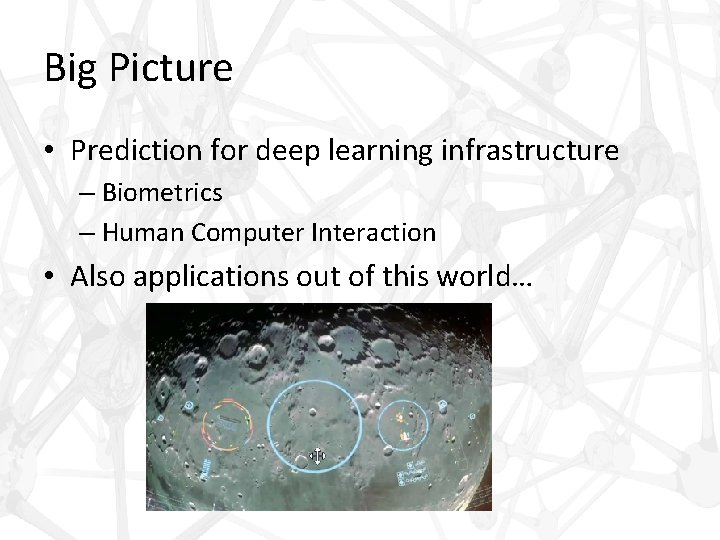
Big Picture • Prediction for deep learning infrastructure – Biometrics – Human Computer Interaction • Also applications out of this world…

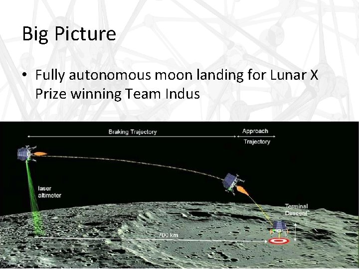
Big Picture • Fully autonomous moon landing for Lunar X Prize winning Team Indus

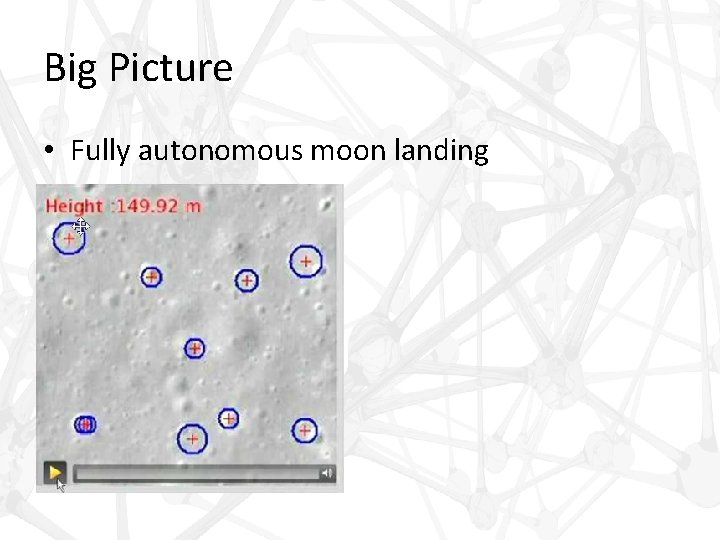
Big Picture • Fully autonomous moon landing

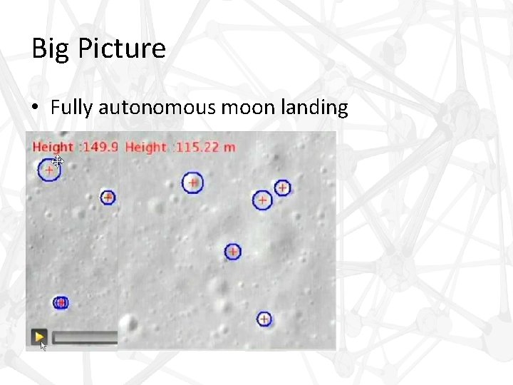
Big Picture • Fully autonomous moon landing

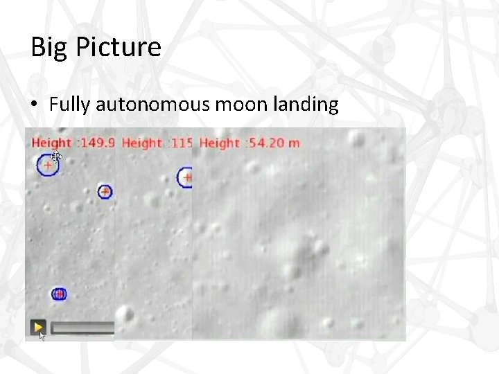
Big Picture • Fully autonomous moon landing

Bibliography • Krizhevsky, A. , Sutskever, I. , and Hinton, G. E. Image. Net classification with deep convolutional neural networks. In NIPS, pp. 1106– 1114, 2012 • Sermanet, P. , Eigen, D. , Zhang, X. , Mathieu, M. , Fergus, R. , and Le. Cun, Y. Over. Feat: Integrated Recognition, Localization and Detection using Convolutional Networks. In Proc. ICLR, 2014 • Szegedy, C. , Liu, W. , Jia, Y. , Sermanet, P. , Reed, S. , Anguelov, D. , Erhan, D. , Vanhoucke, V. , and Rabinovich, A. Going deeper with convolutions. Co. RR, abs/1409. 4842, 2014