Vertical Price Restraints Chapter 18 Vertical Price Restraints

Vertical Price Restraints Chapter 18: Vertical Price Restraints 1

Introduction • Many contractual arrangements between manufacturers – Some restrict rights of retailer • Can’t carry alternative brands • Expected to provide services or to deliver product in a specific amount of time – Some restrict rights of manufacturer • Can’t supply other dealers • Must buy back unsold goods – Some involve restrictions/guidelines on pricing Chapter 18: Vertical Price Restraints 2

Resale Price Maintenance • Resale Price Maintenance is the most important type of vertical price restriction. Under RPM agreement – Retailer agrees to sell at manufactured specified price – RPM agreements have a long and checkered history • In US, Dr. Miles case of 1911 established per se illegality for any and all such agreements • However, Colgate case of 1919 allowed some “wiggle room” • Miller-Tydings (1937) and Mc. Guire (1952) Acts even more supportive in allowing states to enforce RPM contracts – Repeal of Miller-Tydings and Mc. Guire Acts reverted legal status back to (mostly) per se illegal – State Oil v. Khan decision in 1997 allowed rule of reason in RPM agreements setting maximum price – Leegin case applies rule of reason to minimum price Chapter 18: Vertical Price Restraints 3

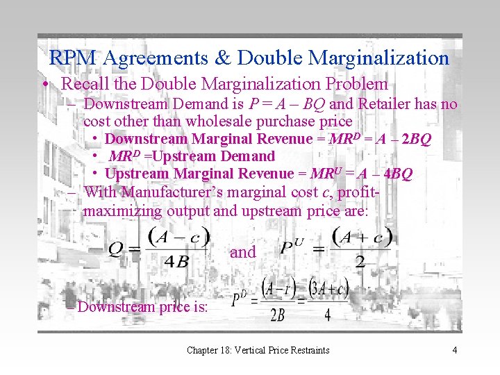
RPM Agreements & Double Marginalization • Recall the Double Marginalization Problem – Downstream Demand is P = A – BQ and Retailer has no cost other than wholesale purchase price • Downstream Marginal Revenue = MRD = A – 2 BQ • MRD =Upstream Demand • Upstream Marginal Revenue = MRU = A – 4 BQ – With Manufacturer’s marginal cost c, profitmaximizing output and upstream price are: and – Downstream price is: Chapter 18: Vertical Price Restraints 4

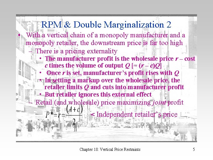
RPM & Double Marginalization 2 • With a vertical chain of a monopoly manufacturer and a monopoly retailer, the downstream price is far too high – There is a pricing externality • The manufacturer profit is the wholesale price r – cost c times the volume of output Q [= (r – c)Q] • Once r is set, manufacturer’s profit rises with Q • In setting a markup over the wholesale price, the retailer limits Q and cuts into manufacturer profit • But retailer ignores this external effect – Retail (and wholesale) price maximizing joint profit < Independent retailer’s price Chapter 18: Vertical Price Restraints 5

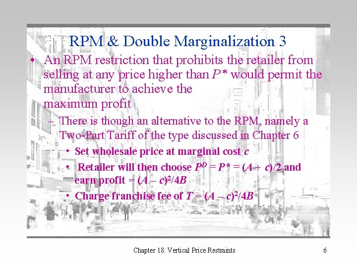
RPM & Double Marginalization 3 • An RPM restriction that prohibits the retailer from selling at any price higher than P* would permit the manufacturer to achieve the maximum profit – There is though an alternative to the RPM, namely a Two-Part Tariff of the type discussed in Chapter 6 • Set wholesale price at marginal cost c • Retailer will then choose PD = P* = (A + c)/2 and earn profit = (A – c)2/4 B • Charge franchise fee of T = (A – c)2/4 B Chapter 18: Vertical Price Restraints 6

RPM & Price Discrimination • An RPM to prevent double marginalization suggests problem is that the retail price is too high • Historical record suggests that perceived problem is often that retail price is too low – Need to find reason(s) for RPM agreements aimed at keeping retail prices high – Retail Price Discrimination may present case where RPM specifying minimum price can help manufacturer Chapter 18: Vertical Price Restraints 7

RPM & Price Discrimination (cont. ) • Suppose retailer operates in two markets – One has less elastic demand (monopolized) – One has elastic demand (due to potential entrant)—retail price P cannot rise above wholesale price r • Manufacturer must use same contract for each – Maximum profit in each market = (A – c)2/4 B achieved at P* = (A + c)/2 – No single price or single two-part tariff can maximize profit from both markets – Unless r = (A + c)/2 in elastic demand market, P* cannot be achieved since in that market P = r – But there is only one contract, so this implies r = (A + c)/2 in inelastic (monopolized) market and so to double marginalization • Solution: write common contract that sets r = c, and imposes RPM minimum price of P=(A+c)/2 Chapter 18: Vertical Price Restraints 8

RPM and Retail Services • So far the retailer has been a totally passive intermediary between manufacturer and consumer • Retailers actually provide additional services: marketing, customer assistance, information, repairs. – These services increase sales – This benefits manufacturers • But offering these services is costly, and also – both services and costs are hard for manufacturer to measure – Retailers interested in her profit not manufacturer’s • How does the manufacturer provide incentives for retailer to offer services? Chapter 18: Vertical Price Restraints 9

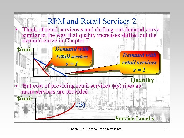
RPM and Retail Services 2 • Think of retail services s and shifting out demand curve similar to the way that quality increases shifted out the demand curve in Chapter 7 Demand with $/unit Demand with retail services s=1 s=2 Quantity • But cost of providing retail services (s) rises as more services are provided $/unit (s) Service Level s Chapter 18: Vertical Price Restraints 10

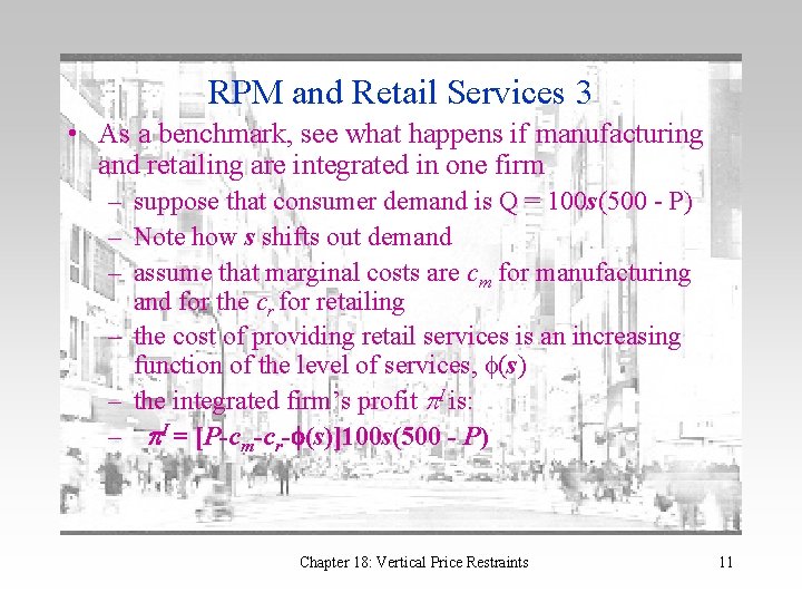
RPM and Retail Services 3 • As a benchmark, see what happens if manufacturing and retailing are integrated in one firm – suppose that consumer demand is Q = 100 s(500 - P) – Note how s shifts out demand – assume that marginal costs are cm for manufacturing and for the cr for retailing – the cost of providing retail services is an increasing function of the level of services, (s) – the integrated firm’s profit I is: – I = [P-cm-cr- (s)]100 s(500 - P) Chapter 18: Vertical Price Restraints 11

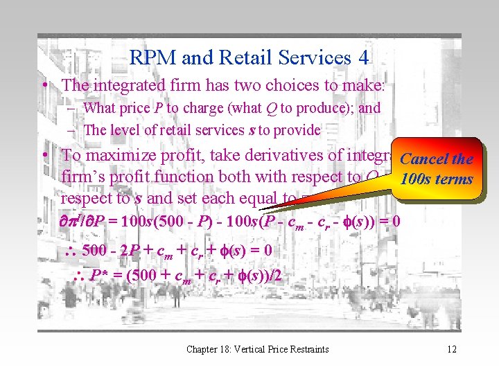
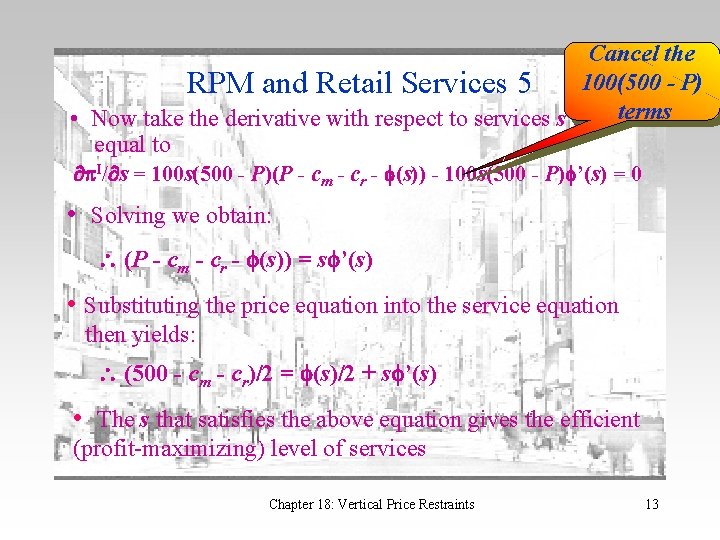
RPM and Retail Services 4 • The integrated firm has two choices to make: – What price P to charge (what Q to produce); and – The level of retail services s to provide • To maximize profit, take derivatives of integrated Cancel the firm’s profit function both with respect to Q and with 100 s terms respect to s and set each equal to zero I/ P = 100 s(500 - P) - 100 s(P - cm - cr - (s)) = 0 500 - 2 P + cm + cr + (s) = 0 P* = (500 + cm + cr + (s))/2 Chapter 18: Vertical Price Restraints 12

Cancel the RPM and Retail Services 5 100(500 - P) terms • Now take the derivative with respect to services s and set it equal to p. I/ s = 100 s(500 - P)(P - cm - cr - (s)) - 100 s(500 - P) ’(s) = 0 • Solving we obtain: (P - cm - cr - (s)) = s ’(s) • Substituting the price equation into the service equation then yields: (500 - cm - cr)/2 = (s)/2 + s ’(s) • The s that satisfies the above equation gives the efficient (profit-maximizing) level of services Chapter 18: Vertical Price Restraints 13

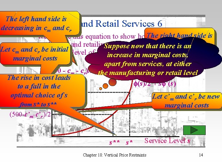
The left hand side is RPM decreasing in cm and cr and Retail Services 6 The right hand • We can use this equation to show changes in theside is in s production and retailing marginal cost (cincreasing and cisr) an affect Suppose now that mthere Let cm and cthe initial level of services r beoptimal increase in marginal costs, marginal costs apart from services, at either (500 - cm - cr)/2 =the (s)/2 + s ’(s) manufacturing or retail level The rise$/unit in cost leads (s)/2 + s ’(s) to a fall in the (500 -cm-c optimal choice of s r)/2 from s* to s** Let c’m and c’r be new marginal costs (500 -c’m-c’r )/2 s** s* Service Level s Chapter 18: Vertical Price Restraints 14

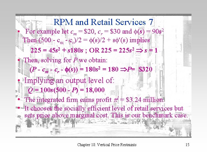
RPM and Retail Services 7 • For example let cm = $20, cr = $30 and (s) = 90 s 2 Then (500 - cm - cr)/2 = (s)/2 + s (s) implies 225 = 45 s 2 + s 180 s ; OR 225 = 225 s 2 s = 1 • Then, solving for P we obtain: (P - cm - cr - (s)) = 180 s 2 = 180 P= $320 • Implying an output level of: Q = 100 s(500 - P) = 18, 000 • The integrated firm earns profit I = $3. 24 million. • It chooses the socially efficient level of retail services but sets price above marginal cost. This is our benchmark case. Chapter 18: Vertical Price Restraints 15

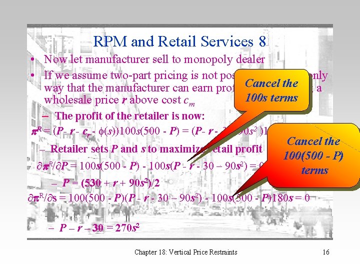
RPM and Retail Services 8 • Now let manufacturer sell to monopoly dealer • If we assume two-part pricing is not possible, then the only the way that the manufacturer can earn profit Cancel is by charging a 100 s terms wholesale price r above cost cm – The profit of the retailer is now: R = (P- r - cr - (s))100 s(500 - P) = (P- r - 30 - 90 s 2 )100 s(500 - P) Cancel the – Retailer sets P and s to maximize retail profit 100(500 - P) R/ P = 100 s(500 - P) - 100 s(P - r - 30 – 90 s 2) = 0 terms – P = (530 + r + 90 s 2)/2 p. R/ s = 100(500 - P)(P - r - 30 – 90 s 2) - 100 s(500 - P)180 s = 0 – P – r – 30 = 270 s 2 Chapter 18: Vertical Price Restraints 16

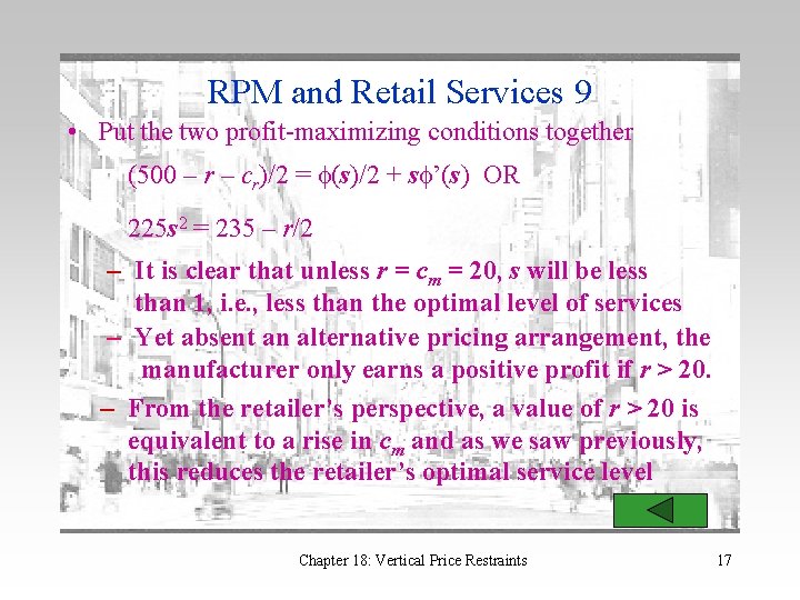
RPM and Retail Services 9 • Put the two profit-maximizing conditions together (500 – r – cr)/2 = (s)/2 + s ’(s) OR 225 s 2 = 235 – r/2 – It is clear that unless r = cm = 20, s will be less than 1, i. e. , less than the optimal level of services – Yet absent an alternative pricing arrangement, the manufacturer only earns a positive profit if r > 20. – From the retailer’s perspective, a value of r > 20 is equivalent to a rise in cm and as we saw previously, this reduces the retailer’s optimal service level Chapter 18: Vertical Price Restraints 17

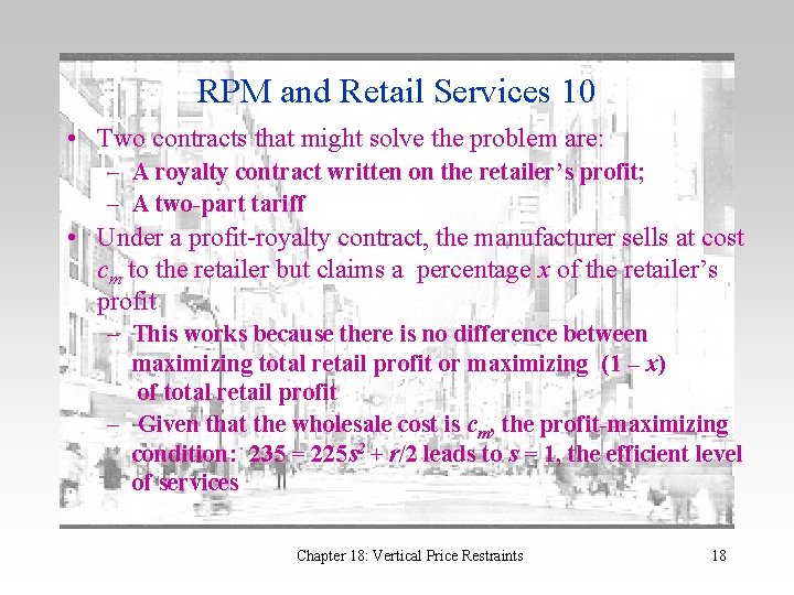
RPM and Retail Services 10 • Two contracts that might solve the problem are: – A royalty contract written on the retailer’s profit; – A two-part tariff • Under a profit-royalty contract, the manufacturer sells at cost cm to the retailer but claims a percentage x of the retailer’s profit – This works because there is no difference between maximizing total retail profit or maximizing (1 – x) of total retail profit – Given that the wholesale cost is cm, the profit-maximizing condition: 235 = 225 s 2 + r/2 leads to s = 1, the efficient level of services Chapter 18: Vertical Price Restraints 18

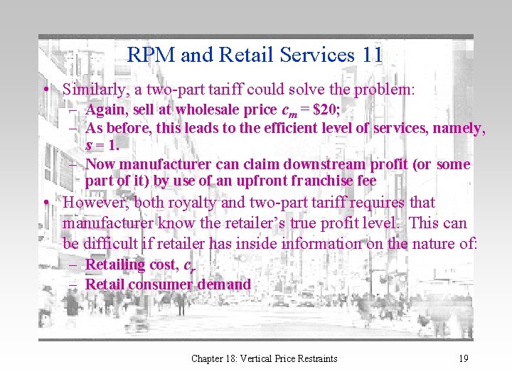
RPM and Retail Services 11 • Similarly, a two-part tariff could solve the problem: – Again, sell at wholesale price cm = $20; – As before, this leads to the efficient level of services, namely, s = 1. – Now manufacturer can claim downstream profit (or some part of it) by use of an upfront franchise fee • However, both royalty and two-part tariff requires that manufacturer know the retailer’s true profit level. This can be difficult if retailer has inside information on the nature of: – Retailing cost, cr – Retail consumer demand Chapter 18: Vertical Price Restraints 19

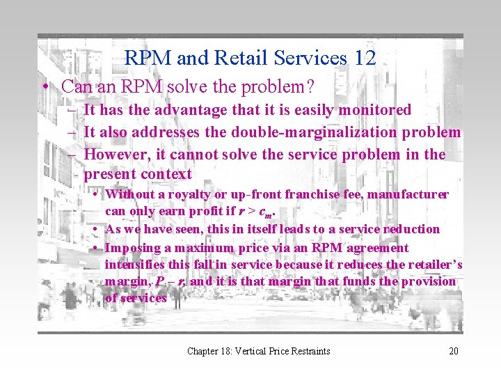
RPM and Retail Services 12 • Can an RPM solve the problem? – It has the advantage that it is easily monitored – It also addresses the double-marginalization problem – However, it cannot solve the service problem in the present context • Without a royalty or up-front franchise fee, manufacturer can only earn profit if r > cm. • As we have seen, this in itself leads to a service reduction • Imposing a maximum price via an RPM agreement intensifies this fall in service because it reduces the retailer’s margin, P – r, and it is that margin that funds the provision of services Chapter 18: Vertical Price Restraints 20

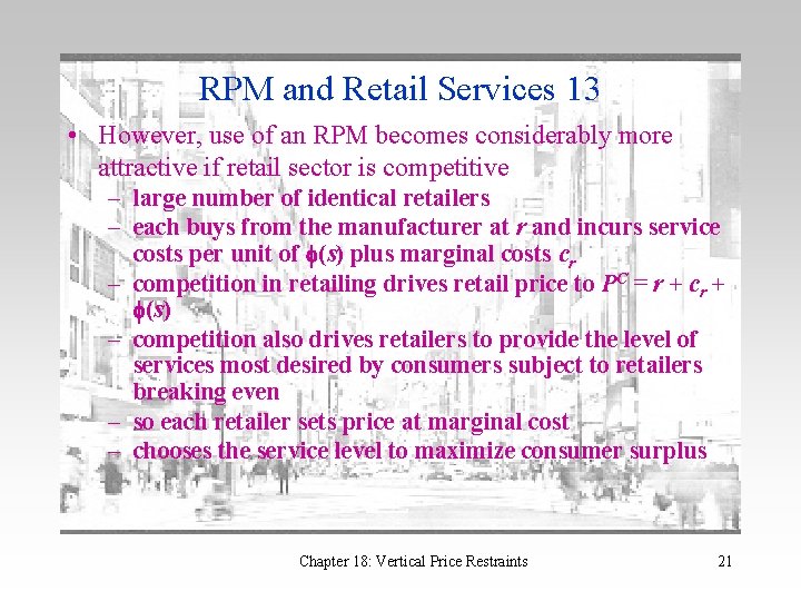
RPM and Retail Services 13 • However, use of an RPM becomes considerably more attractive if retail sector is competitive – large number of identical retailers – each buys from the manufacturer at r and incurs service costs per unit of (s) plus marginal costs cr – competition in retailing drives retail price to PC = r + cr + (s) – competition also drives retailers to provide the level of services most desired by consumers subject to retailers breaking even – so each retailer sets price at marginal cost – chooses the service level to maximize consumer surplus Chapter 18: Vertical Price Restraints 21

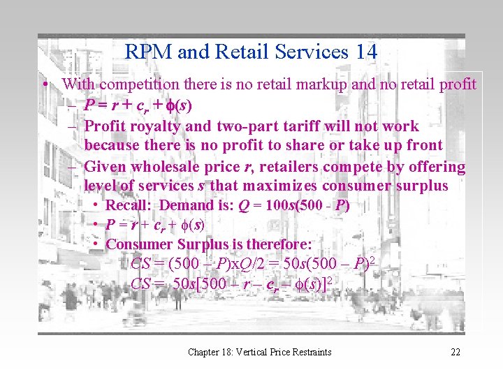
RPM and Retail Services 14 • With competition there is no retail markup and no retail profit – P = r + cr + (s) – Profit royalty and two-part tariff will not work because there is no profit to share or take up front – Given wholesale price r, retailers compete by offering level of services s that maximizes consumer surplus • Recall: Demand is: Q = 100 s(500 - P) • P = r + cr + (s) • Consumer Surplus is therefore: CS = (500 – P)x. Q/2 = 50 s(500 – P)2 CS = 50 s[500 – r – cr – (s)]2 Chapter 18: Vertical Price Restraints 22

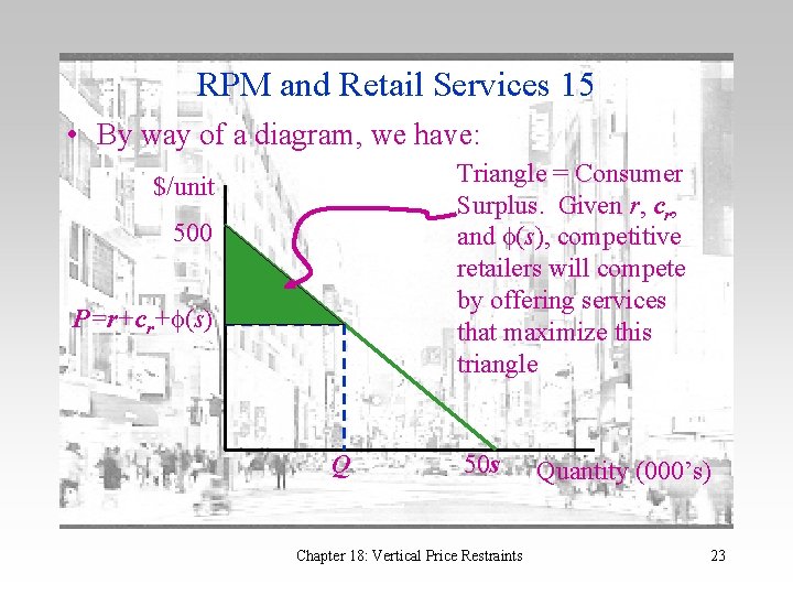
RPM and Retail Services 15 • By way of a diagram, we have: Triangle = Consumer Surplus. Given r, cr, and (s), competitive retailers will compete by offering services that maximize this triangle $/unit 500 P=r+cr+ (s) Q 50 s Chapter 18: Vertical Price Restraints Quantity (000’s) 23

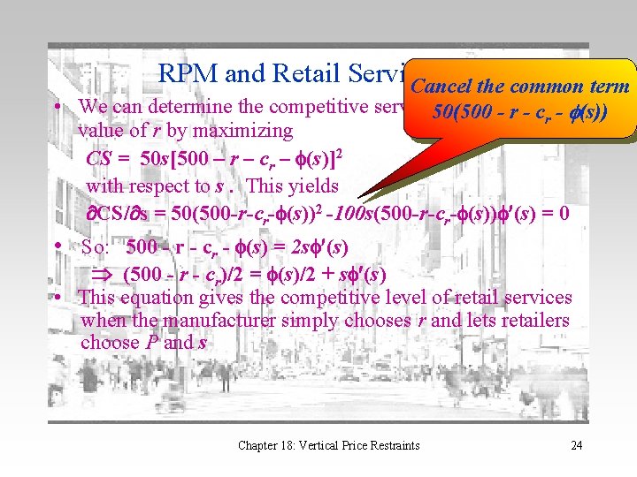
RPM and Retail Services 16 Cancel the common term • We can determine the competitive service 50(500 outcome - rfor - crany - f(s)) value of r by maximizing CS = 50 s[500 – r – cr – (s)]2 with respect to s. This yields CS/ s = 50(500 -r-cr- (s))2 -100 s(500 -r-cr- (s)) (s) = 0 • So: 500 - r - cr - (s) = 2 s (s) (500 - r - cr)/2 = (s)/2 + s (s) • This equation gives the competitive level of retail services when the manufacturer simply chooses r and lets retailers choose P and s Chapter 18: Vertical Price Restraints 24

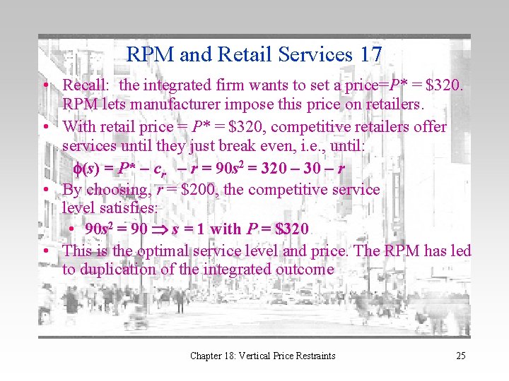
RPM and Retail Services 17 • Recall: the integrated firm wants to set a price=P* = $320. RPM lets manufacturer impose this price on retailers. • With retail price = P* = $320, competitive retailers offer services until they just break even, i. e. , until: (s) = P* – cr – r = 90 s 2 = 320 – 30 – r • By choosing, r = $200, the competitive service level satisfies: • 90 s 2 = 90 s = 1 with P = $320 • This is the optimal service level and price. The RPM has led to duplication of the integrated outcome Chapter 18: Vertical Price Restraints 25

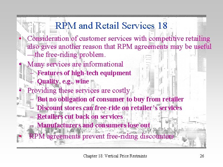
RPM and Retail Services 18 • Consideration of customer services with competitive retailing also gives another reason that RPM agreements may be useful —the free-riding problem. • Many services are informational – Features of high-tech equipment – Quality, e. g. , wine • Providing these services are costly – – But no obligation of consumer to buy from retailer Discount stores can free-ride on retailer’s services Retailers cut back on services Manufacturers and consumers lose out • RPM agreements prevent free-riding discounters Chapter 18: Vertical Price Restraints 26

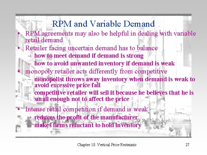
RPM and Variable Demand • RPM agreements may also be helpful in dealing with variable retail demand • Retailer facing uncertain demand has to balance – how to meet demand if demand is strong – how to avoid unwanted inventory if demand is weak • monopoly retailer acts differently from competitive – monopolist throws away inventory when demand is weak to avoid excessive price fall – competitive retailer will sell it because he believes that he is small enough not to affect the price • Intense retail competition if demand is weak – reduces the profit of the manufacturer – makes firms reluctant to hold inventory Chapter 18: Vertical Price Restraints 27

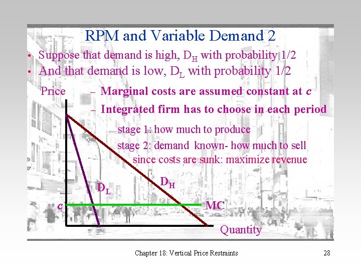
RPM and Variable Demand 2 • Suppose that demand is high, DH with probability 1/2 • And that demand is low, DL with probability 1/2 Price Marginal costs are assumed constant at c – Integrated firm has to choose in each period – stage 1: how much to produce stage 2: demand known- how much to sell since costs are sunk: maximize revenue DL c DH MC Quantity Chapter 18: Vertical Price Restraints 28

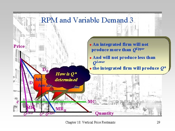
RPM and Variable Demand 3 An integrated firm will not produce more than QUpper Price And will not produce less than QLower the integrated firm will produce Q* DH How is Q* MC = MR with determined MC = MR with DL low demand high demand c MC MRL QLower Q* QUpper MRH Quantity Chapter 18: Vertical Price Restraints 29

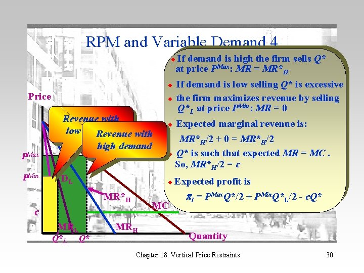
RPM and Variable Demand 4 If demand is high the firm sells Q* at price PMax: MR = MR*H If demand is low selling Q* is excessive the firm maximizes revenue by selling Q*L at price PMin: MR = 0 Expected marginal revenue is: Price PMax PMin Revenue with low demand Revenue with DHhigh demand DL Expected MR*H MC c MRL Q*L MR*H/2 + 0 = MR*H/2 Q* is such that expected MR = MC. So, MR*H/2 = c Q* MRH profit is I = PMax. Q*/2 + PMin. Q*L/2 - c. Q* Quantity Chapter 18: Vertical Price Restraints 30

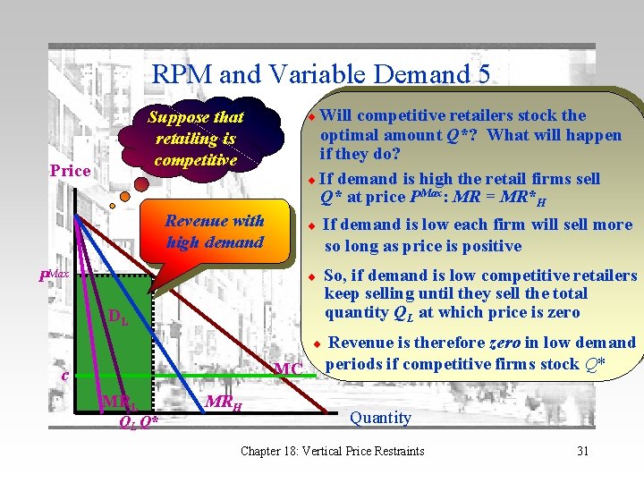
RPM and Variable Demand 5 Will competitive retailers stock the optimal amount Q*? What will happen if they do? If demand is high the retail firms sell Q* at price PMax: MR = MR*H Suppose that retailing is competitive Price Revenue with high demand DH PMax If demand is low each firm will sell more so long as price is positive So, if demand is low competitive retailers keep selling until they sell the total quantity QL at which price is zero DL MC c MRL QL Q* MRH Revenue is therefore zero in low demand periods if competitive firms stock Q* Quantity Chapter 18: Vertical Price Restraints 31

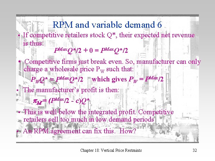
RPM and variable demand 6 • If competitive retailers stock Q*, their expected net revenue is thus: PMax. Q*/2 + 0 = PMax. Q*/2 • Competitive firms just break even. So, manufacturer can only charge a wholesale price PW such that: PWQ* = PMax. Q*/2 which gives PW = PMax/2 • The manufacturer’s profit is then: M = (PMax/2 - c)Q* • This is well below the integrated profit. Competitive retailers sell too much in low demand periods • An RPM agreement can fix this. How? Chapter 18: Vertical Price Restraints 32

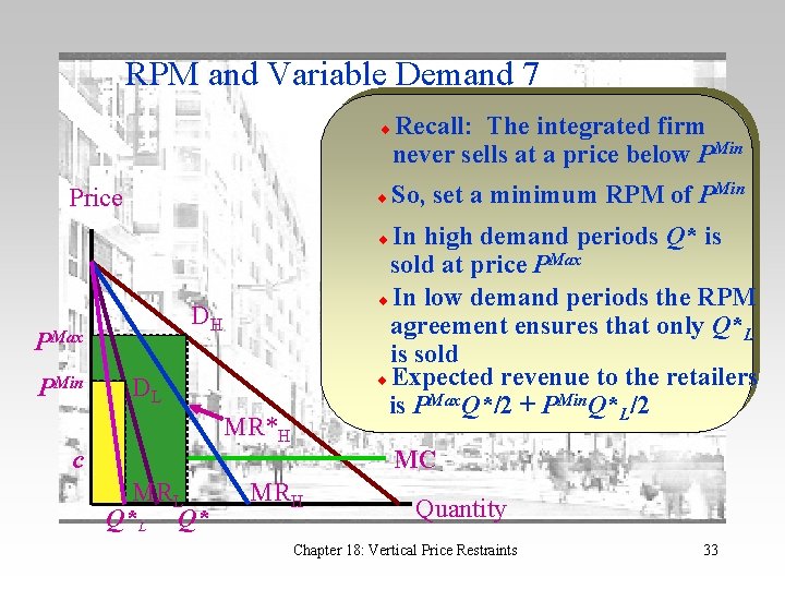
RPM and Variable Demand 7 Price Recall: The integrated firm never sells at a price below PMin So, set a minimum RPM of PMin In high demand periods Q* is sold at price PMax In low demand periods the RPM agreement ensures that only Q*L is sold Expected revenue to the retailers is PMax. Q*/2 + PMin. Q*L/2 DH PMax PMin DL MR*H c MRL Q* MC MRH Quantity Chapter 18: Vertical Price Restraints 33

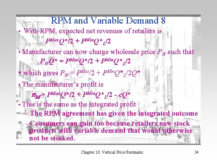
RPM and Variable Demand 8 • With RPM, expected net revenues of retailers is PMax. Q*/2 + PMin. Q*L/2 • Manufacturer can now charge wholesale price PW such that: PWQ* = PMax. Q*/2 + PMin. Q*L/2 • which gives PW = PMax/2 + PMin. Q*L/2 Q* • The manufacturer’s profit is M = PMax. Q*/2 + PMin. Q*L/2 - c. Q* • This is the same as the integrated profit – The RPM agreement has given the integrated outcome – Consumers can gain too because retailers now stock products with variable demand that would otherwise not be stocked. Chapter 18: Vertical Price Restraints 34