VECTORS AND MATRICES Vectors and matrices are used

VECTORS AND MATRICES

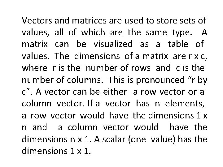
Vectors and matrices are used to store sets of values, all of which are the same type. A matrix can be visualized as a table of values. The dimensions of a matrix are r x c, where r is the number of rows and c is the number of columns. This is pronounced “r by c”. A vector can be either a row vector or a column vector. If a vector has n elements, a row vector would have the dimensions 1 x n and a column vector would have the dimensions n x 1. A scalar (one value) has the dimensions 1 x 1.

MATLAB is written to work with matrices; the name MATLAB is short for matrix laboratory. A vector in MATLAB is equivalent to what is called a one-dimensional array in other languages. A matrix is equivalent to a two-dimensional array.

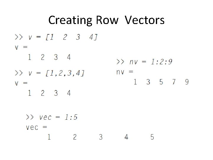
Creating Row Vectors

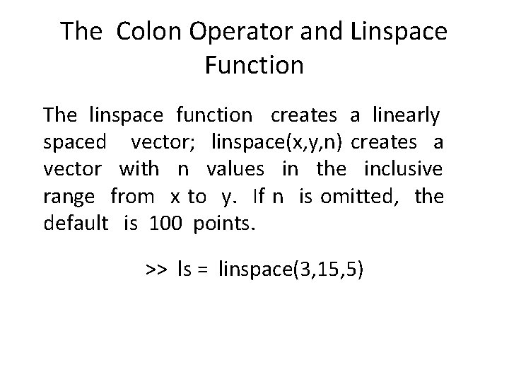
The Colon Operator and Linspace Function The linspace function creates a linearly spaced vector; linspace(x, y, n) creates a vector with n values in the inclusive range from x to y. If n is omitted, the default is 100 points. >> ls = linspace(3, 15, 5)

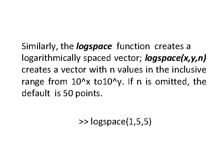
Similarly, the logspace function creates a logarithmically spaced vector; logspace(x, y, n) creates a vector with n values in the inclusive range from 10^x to 10^y. If n is omitted, the default is 50 points. >> logspace(1, 5, 5)

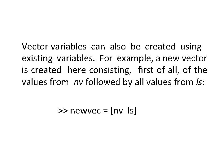
Vector variables can also be created using existing variables. For example, a new vector is created here consisting, first of all, of the values from nv followed by all values from ls: >> newvec = [nv ls]

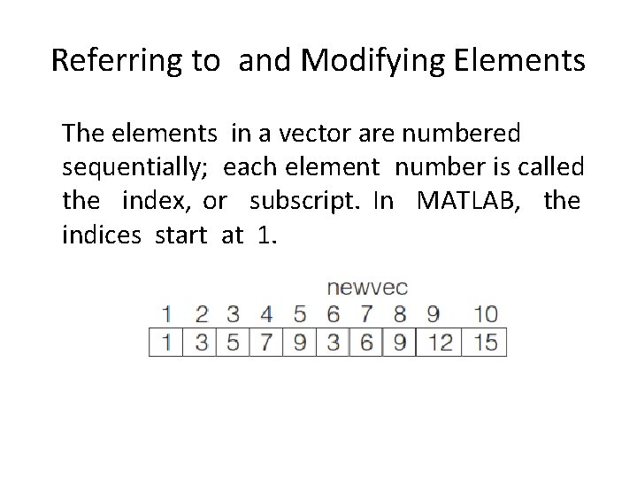
Referring to and Modifying Elements The elements in a vector are numbered sequentially; each element number is called the index, or subscript. In MATLAB, the indices start at 1.

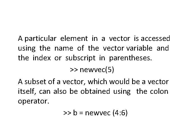
A particular element in a vector is accessed using the name of the vector variable and the index or subscript in parentheses. >> newvec(5) A subset of a vector, which would be a vector itself, can also be obtained using the colon operator. >> b = newvec (4: 6)

>> newvec ([1 10 5]) The value stored in a vector element can be changed by specifying the index or subscript. >> b(2)=11 >> rv(6)=13

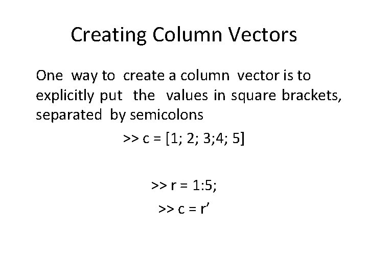
Creating Column Vectors One way to create a column vector is to explicitly put the values in square brackets, separated by semicolons >> c = [1; 2; 3; 4; 5] >> r = 1: 5; >> c = r’

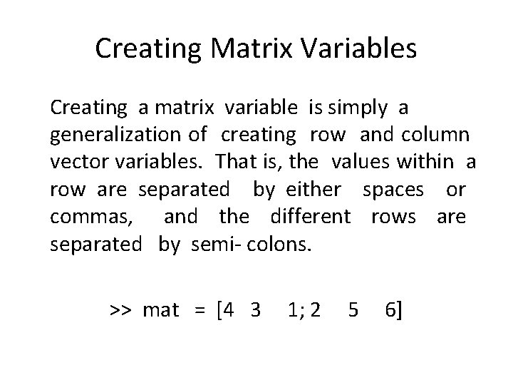
Creating Matrix Variables Creating a matrix variable is simply a generalization of creating row and column vector variables. That is, the values within a row are separated by either spaces or commas, and the different rows are separated by semi- colons. >> mat = [4 3 1; 2 5 6]

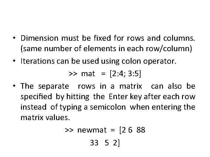
• Dimension must be fixed for rows and columns. (same number of elements in each row/column) • Iterations can be used using colon operator. >> mat = [2: 4; 3: 5] • The separate rows in a matrix can also be specified by hitting the Enter key after each row instead of typing a semicolon when entering the matrix values. >> newmat = [2 6 88 33 5 2]

Matrices of random numbers can be created using the rand function. If a single value n is passed to rand, an n x n matrix will be created, or passing two arguments will specify the number of rows and columns: >> rand(2) >> rand(1, 3)

Matrices of random integers can be generated using randi; after the range is passed, the dimensions of the matrix are passed. >> randi([5, 10], 2) >> randi([10, 30], 2, 3)

MATLAB also has several functions that create special matrices. >> zeros(3) >> ones(2, 4)

Referring to and Modifying Matrix Elements To refer to matrix elements, the row and then the column subscripts are given in parentheses >> mat = [2: 4; 3: 5] >> mat(2, 3) It is also possible to refer to a subset of a matrix. >> mat(1: 2, 2: 3)

• Using just one colon by itself for the row subscript means all rows, regardless of how many, and using a colon for the column subscript means all columns. >> mat(1, : ) >> mat(: , 2) • If a single index is used with a matrix, MATLAB unwinds the matrix column by column.

• An individual element in a matrix can be modified by assigning a new value to it. >> mat = [2: 4; 3: 5]; >> mat(1, 2) = 11 • An entire row or column could also be changed. >> mat(2, : ) = 5: 7

• To extend a matrix an individual element could not be added, however an entire row or column could be added. >> mat(: , 4) = [9 2]‘ • Just as we saw with vectors, if there is a gap between the current matrix and the row or column being added, MATLAB will fill in with zeros. >> mat(4, : ) = 2: 2: 8

Dimensions • The length and size functions in MATLAB are used to find dimensions of vectors and matrices. The length function will return either the number of rows or the number of columns, whichever is largest >> vec = -2: 1 >> length(vec) >> size(vec) >> [r, c] = size(mat)

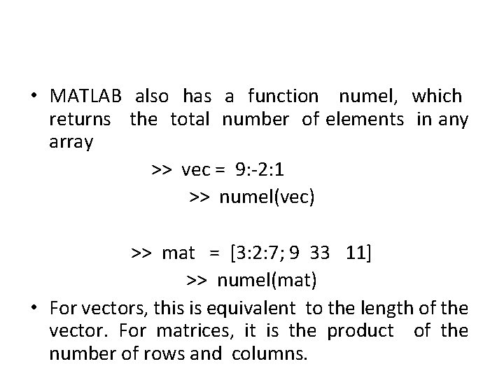
• MATLAB also has a function numel, which returns the total number of elements in any array >> vec = 9: -2: 1 >> numel(vec) >> mat = [3: 2: 7; 9 33 11] >> numel(mat) • For vectors, this is equivalent to the length of the vector. For matrices, it is the product of the number of rows and columns.

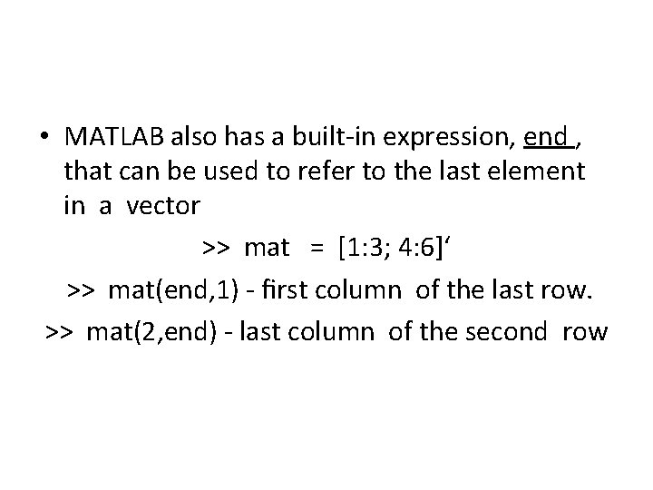
• MATLAB also has a built-in expression, end , that can be used to refer to the last element in a vector >> mat = [1: 3; 4: 6]‘ >> mat(end, 1) - first column of the last row. >> mat(2, end) - last column of the second row

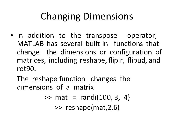
Changing Dimensions • In addition to the transpose operator, MATLAB has several built-in functions that change the dimensions or configuration of matrices, including reshape, fliplr, flipud, and rot 90. The reshape function changes the dimensions of a matrix >> mat = randi(100, 3, 4) >> reshape(mat, 2, 6)

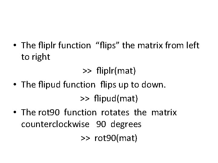
• The fliplr function “flips” the matrix from left to right >> fliplr(mat) • The flipud function flips up to down. >> flipud(mat) • The rot 90 function rotates the matrix counterclockwise 90 degrees >> rot 90(mat)

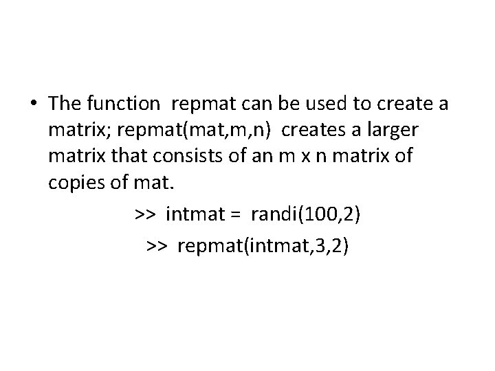
• The function repmat can be used to create a matrix; repmat(mat, m, n) creates a larger matrix that consists of an m x n matrix of copies of mat. >> intmat = randi(100, 2) >> repmat(intmat, 3, 2)

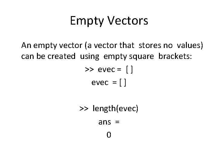
Empty Vectors An empty vector (a vector that stores no values) can be created using empty square brackets: >> evec = [ ] >> length(evec) ans = 0

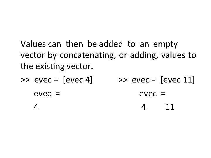
Values can then be added to an empty vector by concatenating, or adding, values to the existing vector. >> evec = [evec 4] >> evec = [evec 11] evec = 4 4 11

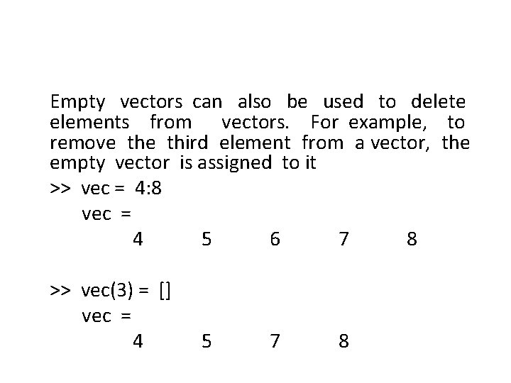
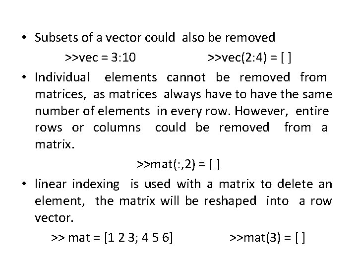
Empty vectors can also be used to delete elements from vectors. For example, to remove third element from a vector, the empty vector is assigned to it >> vec = 4: 8 vec = 4 5 6 7 8 >> vec(3) = [] vec = 4 5 7 8

• Subsets of a vector could also be removed >>vec = 3: 10 >>vec(2: 4) = [ ] • Individual elements cannot be removed from matrices, as matrices always have to have the same number of elements in every row. However, entire rows or columns could be removed from a matrix. >>mat(: , 2) = [ ] • linear indexing is used with a matrix to delete an element, the matrix will be reshaped into a row vector. >> mat = [1 2 3; 4 5 6] >>mat(3) = [ ]

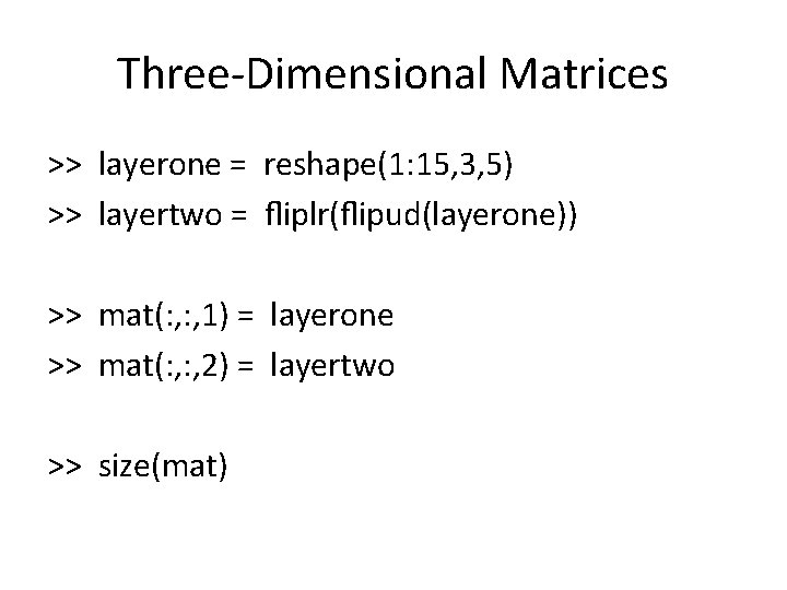
Three-Dimensional Matrices >> layerone = reshape(1: 15, 3, 5) >> layertwo = fliplr(flipud(layerone)) >> mat(: , 1) = layerone >> mat(: , 2) = layertwo >> size(mat)

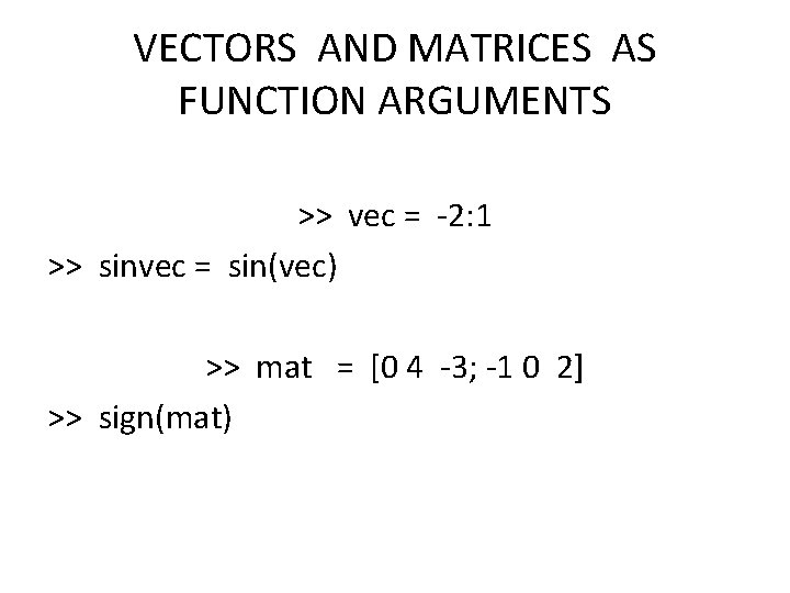
VECTORS AND MATRICES AS FUNCTION ARGUMENTS >> vec = -2: 1 >> sinvec = sin(vec) >> mat = [0 4 -3; -1 0 2] >> sign(mat)

>> vec 1 = 1: 5; >> vec 2 = [3 5 8 2]; >> min(vec 1) >> max(vec 2) >> sum(vec 1) >> prod(vec 2) >> cumsum(vec 1) >> cumsum(vec 2) >> cumprod(vec 1)

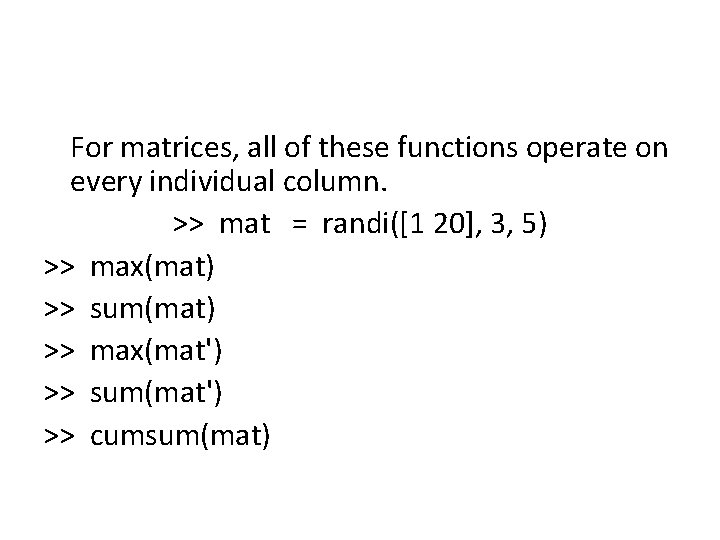
For matrices, all of these functions operate on every individual column. >> mat = randi([1 20], 3, 5) >> max(mat) >> sum(mat) >> max(mat') >> sum(mat') >> cumsum(mat)

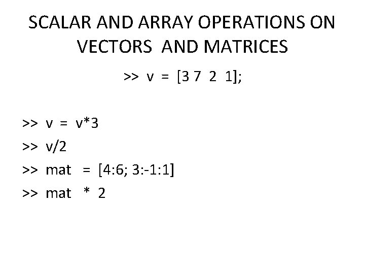
SCALAR AND ARRAY OPERATIONS ON VECTORS AND MATRICES >> v = [3 7 2 1]; >> v = v*3 >> v/2 >> mat = [4: 6; 3: -1: 1] >> mat * 2

>> v 1 = 2: 5 >> v 2 = [33 11 5 1] >> v 1 + v 2 >> mata = [5: 8; 9: -2: 3] >> matb = reshape(1: 8, 2, 4) >> mata – matb

Exponentiation operator Array multiplication and Division >> v = [3 7 2 1]; >> v . ^ 2 >> v 1 = 2: 5 >> v 2 = [33 11 5 1] >> v 1 . * v 2 >> mata. / matb

MATRIX MULTIPLICATION >> A = [ 3 8 0; 1 2 5] A = 3 8 0 1 2 5 >> B = [ 1 2 3 1; 4 5 1 2; 0 2 3 0] B = 1 2 3 1 4 5 1 2 0 2 3 0 >> C= A*B C = 35 46 17 19 9 22 20 5 >>

Matrix Multiplication for Vectors >> c = [5 3 7 1]'; >> r = [6 2 3 4]; >> r*c >> c*r ans = 61 30 15 20 18 6 9 12 42 14 21 28 6 2 3 4 >>

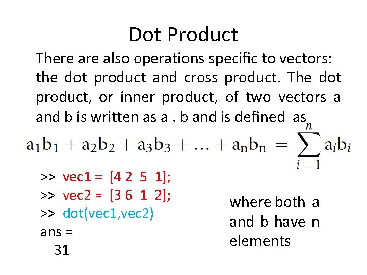
Dot Product There also operations specific to vectors: the dot product and cross product. The dot product, or inner product, of two vectors a and b is written as a. b and is defined as >> vec 1 = [4 2 5 1]; >> vec 2 = [3 6 1 2]; >> dot(vec 1, vec 2) ans = 31 where both a and b have n elements

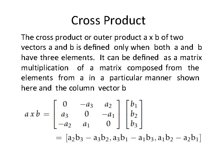
Cross Product The cross product or outer product a x b of two vectors a and b is defined only when both a and b have three elements. It can be defined as a matrix multiplication of a matrix composed from the elements from a in a particular manner shown here and the column vector b

>> vec 1 = [4 2 5]; >> vec 2 = [3 6 1]; >> cross(vec 1, vec 2) ans = -28 11 18

LOGICAL VECTORS >> vec = [5 9 3 4 6 11]; >> isg = vec > 5 isg = 0 1 0 0 1 1 >> sum(isg) %sum of vectors greater than 5 ans = 3 >> vec(isg) % shows vectors that are greater than 5 ans = 9 6 11

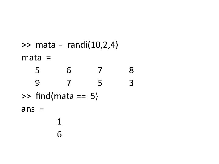
>> mata = randi(10, 2, 4) mata = 5 6 7 8 9 7 5 3 >> find(mata == 5) ans = 1 6

THE DIFF FUNCTION >> diff([4 7 15 32]) ans = 3 8 17 >> mat = randi(20, 2, 3) mat = 17 3 13 19 2 >> diff(mat) ans = 2 16 -11

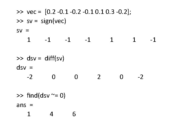
>> vec = [0. 2 -0. 1 -0. 2 -0. 1 0. 3 -0. 2]; >> sv = sign(vec) sv = 1 -1 1 1 -1 >> dsv = diff(sv) dsv = -2 0 0 2 0 -2 >> find(dsv ~= 0) ans = 1 4 6

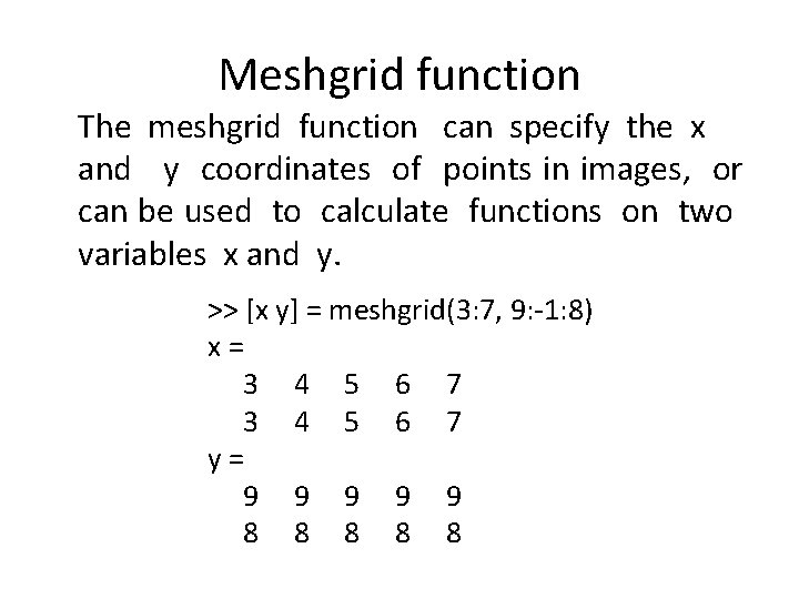
Meshgrid function The meshgrid function can specify the x and y coordinates of points in images, or can be used to calculate functions on two variables x and y. >> [x y] = meshgrid(3: 7, 9: -1: 8) x = 3 4 5 6 7 y = 9 9 9 8 8 8