Vector Space Classification Adapted from Lectures by Raymond

Vector Space Classification Adapted from Lectures by Raymond Mooney and Barbara Rosario Prasad L 11 Classify 1

Text Classification n Today: n Introduction to Text Classification n n K Nearest Neighbors Decision boundaries Vector space classification using centroids Decision Trees (briefly) Later n More text classification n n Support Vector Machines Text-specific issues in classification 2

Recall: Vector Space Representation n Each document is a vector, one component for each term (= word). Normalize to unit length. High-dimensional vector space: n n n Terms are axes 10, 000+ dimensions, or even 100, 000+ Docs are vectors in this space 3

Classification Using Vector Spaces n n n Each training doc a point (vector) labeled by its topic (= class) Hypothesis: docs of the same class form a contiguous region of space We define surfaces to delineate classes in space 4

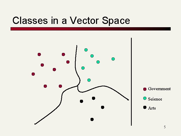
Classes in a Vector Space Government Science Arts 5

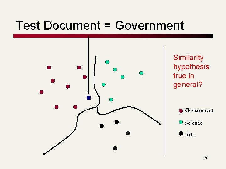
Test Document = Government Similarity hypothesis true in general? Government Science Arts 6

k Nearest Neighbor Classification 7

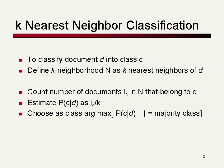
k Nearest Neighbor Classification n n To classify document d into class c Define k-neighborhood N as k nearest neighbors of d Count number of documents ic in N that belong to c Estimate P(c|d) as ic/k Choose as class arg maxc P(c|d) [ = majority class] 8

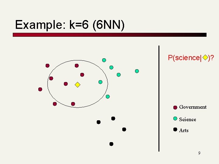
Example: k=6 (6 NN) P(science| )? Government Science Arts 9

Nearest-Neighbor Learning Algorithm n n Learning is just storing the representations of the training examples in D. Testing instance x: n n Compute similarity between x and all examples in D. Assign x the category of the most similar example in D. Does not explicitly compute a generalization or category prototypes. Also called: n Case-based learning, Memory-based learning, Lazy learning 10

K Nearest-Neighbor n Using only the closest example (k=1) to determine the category is subject to errors due to: n n A single atypical example. Noise in the category label of a single training example. More robust alternative is to find the k mostsimilar examples and return the majority category of these k examples. Value of k is typically odd to avoid ties; 3 and 5 are most common. 11

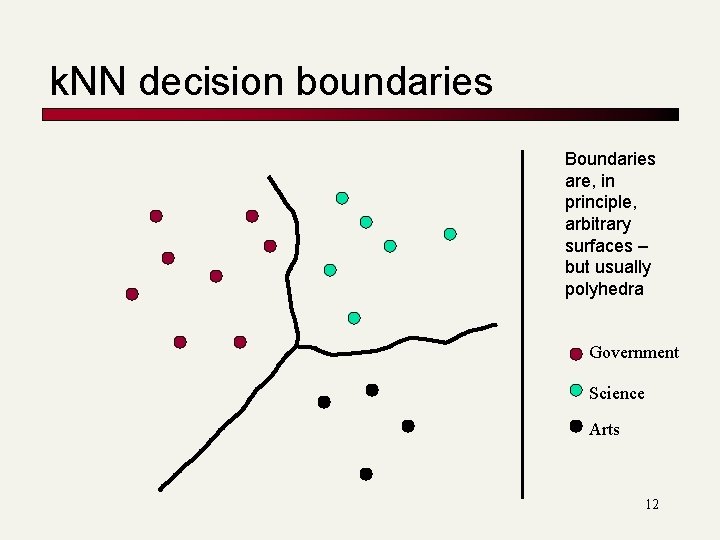
k. NN decision boundaries Boundaries are, in principle, arbitrary surfaces – but usually polyhedra Government Science Arts 12

Similarity Metrics n Nearest neighbor method depends on a similarity (or distance) metric. n Simplest for continuous m-dimensional instance space is Euclidean distance. n Simplest for m-dimensional binary instance space is Hamming distance (number of feature values that differ). n For text, cosine similarity of tf. idf weighted vectors is typically most effective. 13

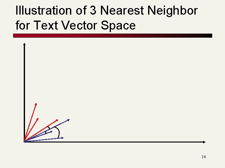
Illustration of 3 Nearest Neighbor for Text Vector Space 14

Nearest Neighbor with Inverted Index n n Naively finding nearest neighbors requires a linear search through |D| documents in collection But determining k nearest neighbors is the same as determining the k best retrievals using the test document as a query to a database of training documents. Use standard vector space inverted index methods to find the k nearest neighbors. Testing Time: O(B|Vt|) where B is the average number of training documents in which a testdocument word appears. n Typically B << |D| 15

k. NN: Discussion n n No feature selection necessary Scales well with large number of classes n n Classes can influence each other n n n Don’t need to train n classifiers for n classes Small changes to one class can have ripple effect Scores can be hard to convert to probabilities No training necessary n Actually: perhaps not true. (Data editing, etc. ) 16

Decision Boundaries Classification 17

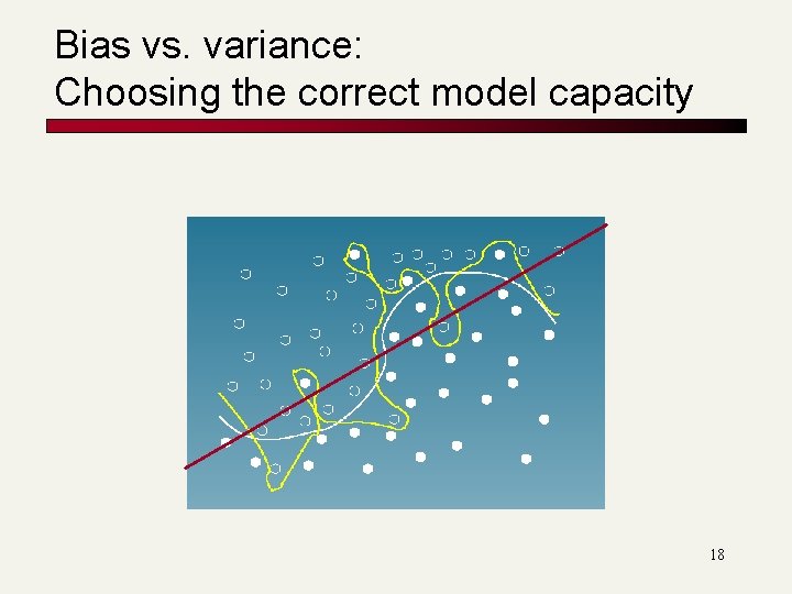
Bias vs. variance: Choosing the correct model capacity 18

Binary Classification n Consider 2 class problems n n n Deciding between two classes, perhaps, government and non-government [one-versus-rest classification] How do we define (and find) the separating surface? How do we test which region a test doc is in? 19

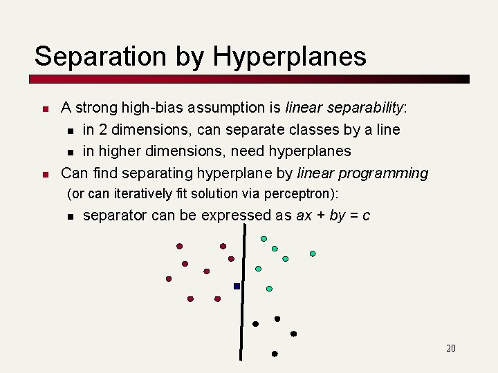
Separation by Hyperplanes n n A strong high-bias assumption is linear separability: n in 2 dimensions, can separate classes by a line n in higher dimensions, need hyperplanes Can find separating hyperplane by linear programming (or can iteratively fit solution via perceptron): n separator can be expressed as ax + by = c 20

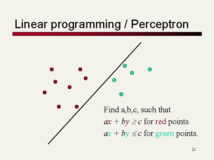
Linear programming / Perceptron Find a, b, c, such that ax + by c for red points ax + by c for green points. 21

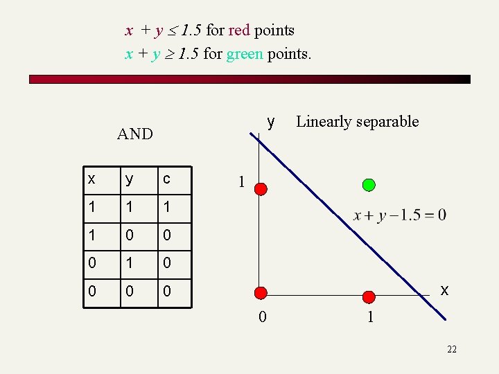
x + y 1. 5 for red points x + y 1. 5 for green points. y AND x y c 1 1 0 0 0 1 0 0 Linearly separable 1 x 0 1 22

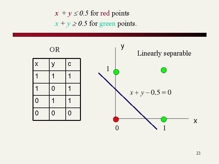
x + y 0. 5 for red points x + y 0. 5 for green points. y OR x y c 1 1 0 0 0 Linearly separable 1 0 1 x 23

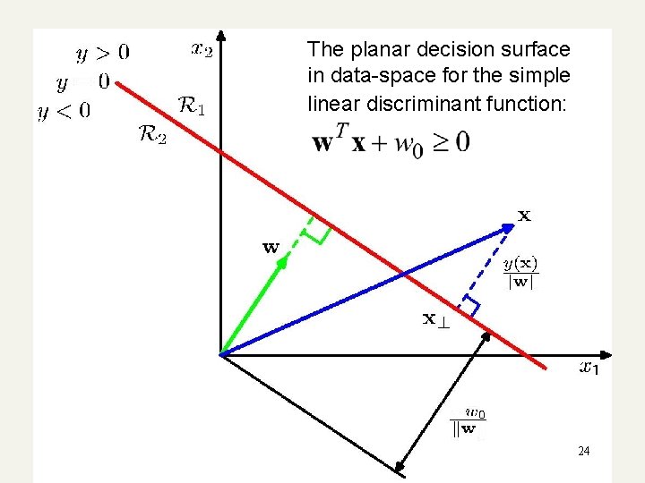
The planar decision surface in data-space for the simple linear discriminant function: 24

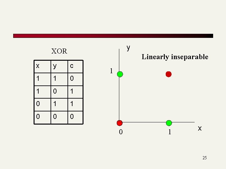
y XOR Linearly inseparable x y c 1 1 0 1 0 1 1 0 0 0 1 x 25

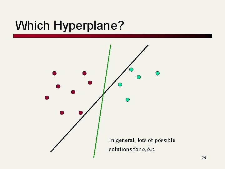
Which Hyperplane? In general, lots of possible solutions for a, b, c. 26

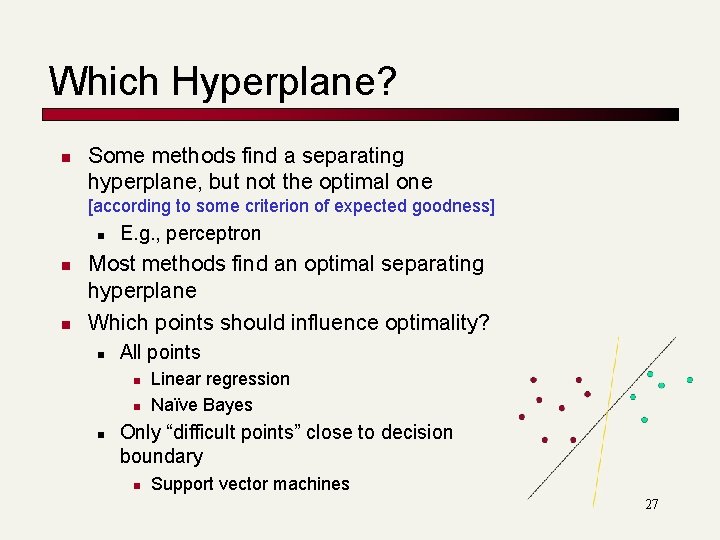
Which Hyperplane? n Some methods find a separating hyperplane, but not the optimal one [according to some criterion of expected goodness] n n n E. g. , perceptron Most methods find an optimal separating hyperplane Which points should influence optimality? n All points n n n Linear regression Naïve Bayes Only “difficult points” close to decision boundary n Support vector machines 27

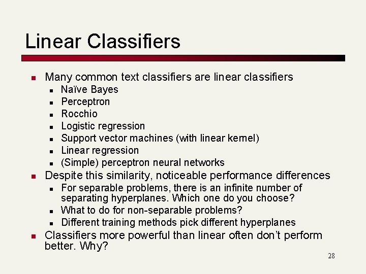
Linear Classifiers n Many common text classifiers are linear classifiers n n n n Despite this similarity, noticeable performance differences n n Naïve Bayes Perceptron Rocchio Logistic regression Support vector machines (with linear kernel) Linear regression (Simple) perceptron neural networks For separable problems, there is an infinite number of separating hyperplanes. Which one do you choose? What to do for non-separable problems? Different training methods pick different hyperplanes Classifiers more powerful than linear often don’t perform better. Why? 28

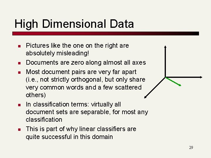
High Dimensional Data n n n Pictures like the on the right are absolutely misleading! Documents are zero along almost all axes Most document pairs are very far apart (i. e. , not strictly orthogonal, but only share very common words and a few scattered others) In classification terms: virtually all document sets are separable, for most any classification This is part of why linear classifiers are quite successful in this domain 29

More Than Two Classes n Any-of or multivalue classification n n Classes are independent of each other. A document can belong to 0, 1, or >1 classes. Decompose into n binary problems Quite common for documents One-of or multinomial or polytomous classification n Classes are mutually exclusive. Each document belongs to exactly one class E. g. , digit recognition is polytomous classification n Digits are mutually exclusive 30

Set of Binary Classifiers: Any of n n Build a separator between each class and its complementary set (docs from all other classes). Given test doc, evaluate it for membership in each class. Apply decision criterion of classifiers independently Done n Sometimes you could do better by considering dependencies between categories 31

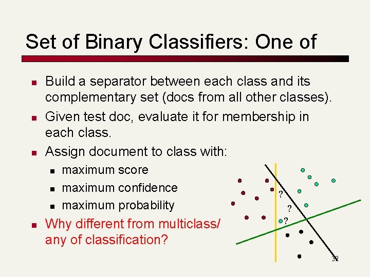
Set of Binary Classifiers: One of n n n Build a separator between each class and its complementary set (docs from all other classes). Given test doc, evaluate it for membership in each class. Assign document to class with: n n maximum score maximum confidence maximum probability Why different from multiclass/ any of classification? ? ? ? 32

Classification using Centroids 33

Based on Rocchio Method n n n Use standard TF/IDF weighted vectors to represent text documents For each category, compute a prototype vector by summing the vectors of the training documents in the category. n Prototype = centroid of members of class Assign test documents to the category with the closest prototype vector based on cosine similarity. 34

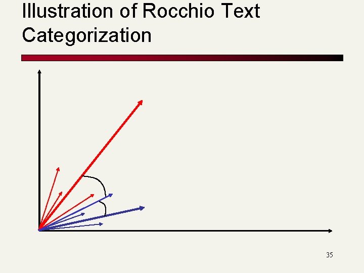
Illustration of Rocchio Text Categorization 35

Rocchio Properties n n Forms a simple generalization of the examples in each class (a prototype). Prototype vector does not need to be averaged or otherwise normalized for length since cosine similarity is insensitive to vector length. Classification is based on similarity to class prototypes. Does not guarantee classifications are consistent with the given training data. 36

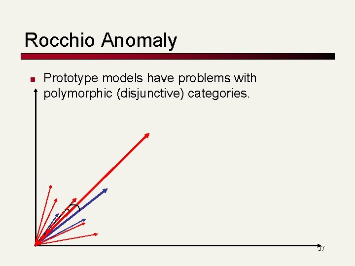
Rocchio Anomaly n Prototype models have problems with polymorphic (disjunctive) categories. 37

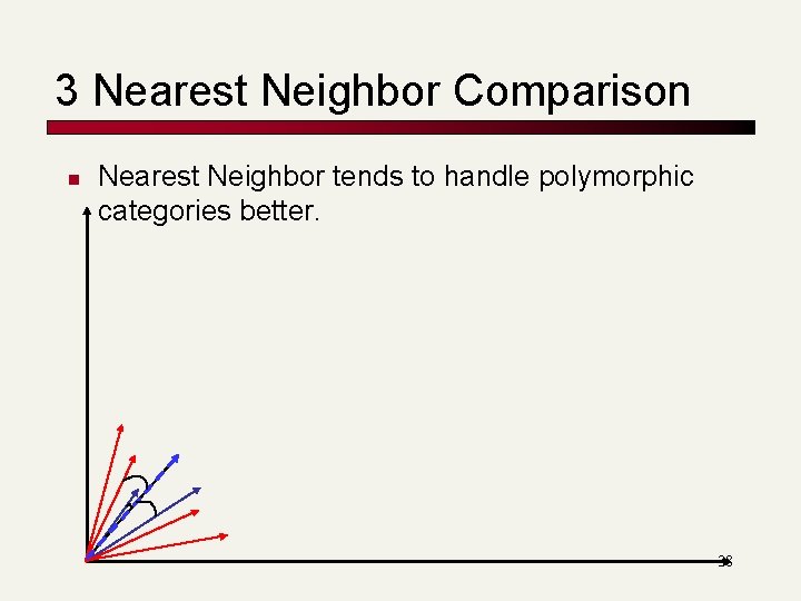
3 Nearest Neighbor Comparison n Nearest Neighbor tends to handle polymorphic categories better. 38

SKIP WHAT FOLLOWS 39

Decision Tree Classification n n n Tree with internal nodes labeled by terms Branches are labeled by tests on the weight that the term has Leaves are labeled by categories Classifier categorizes document by descending tree following tests to leaf The label of the leaf node is then assigned to the document Most decision trees are binary trees (never disadvantageous; may require extra internal nodes) DT make good use of a few high-leverage features 40

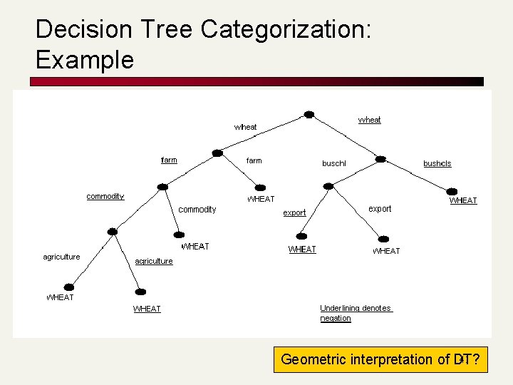
Decision Tree Categorization: Example 41 Geometric interpretation of DT?

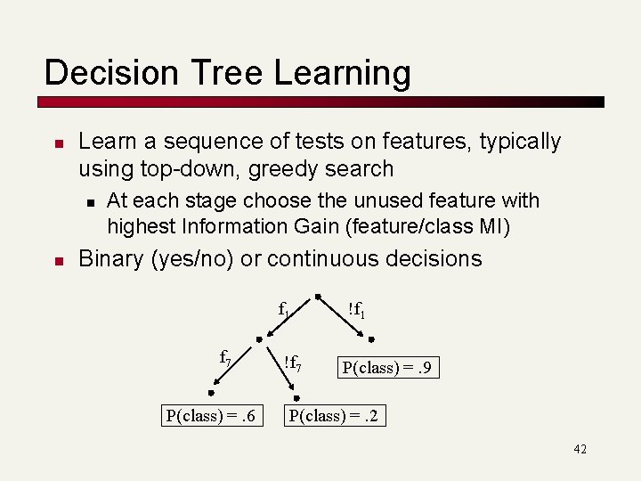
Decision Tree Learning n Learn a sequence of tests on features, typically using top-down, greedy search n n At each stage choose the unused feature with highest Information Gain (feature/class MI) Binary (yes/no) or continuous decisions f 7 P(class) =. 6 f 1 !f 7 P(class) =. 9 P(class) =. 2 42

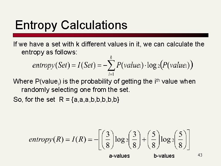
Entropy Calculations If we have a set with k different values in it, we can calculate the entropy as follows: Where P(valuei) is the probability of getting the ith value when randomly selecting one from the set. So, for the set R = {a, a, a, b, b, b} a-values b-values 43

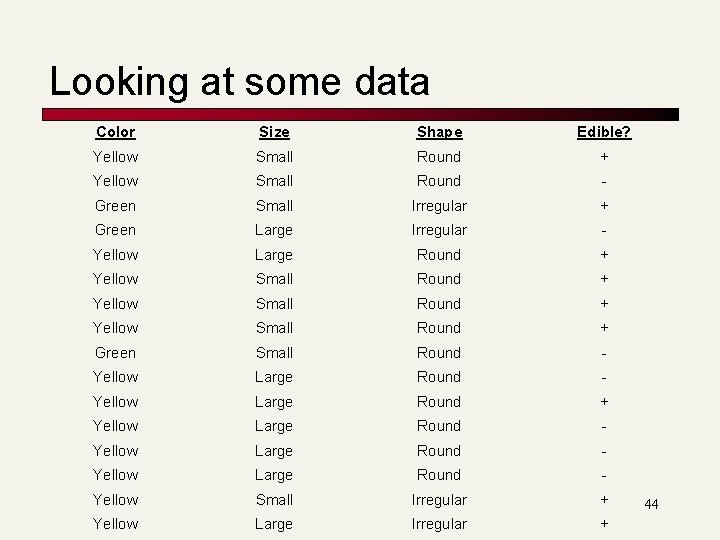
Looking at some data Color Size Shape Edible? Yellow Small Round + Yellow Small Round - Green Small Irregular + Green Large Irregular - Yellow Large Round + Yellow Small Round + Green Small Round - Yellow Large Round + Yellow Large Round - Yellow Small Irregular + Yellow Large Irregular + 44

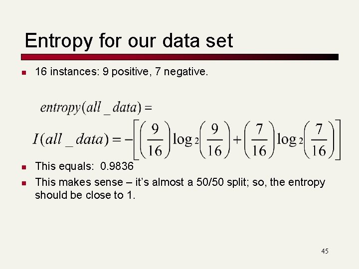
Entropy for our data set n n n 16 instances: 9 positive, 7 negative. This equals: 0. 9836 This makes sense – it’s almost a 50/50 split; so, the entropy should be close to 1. 45

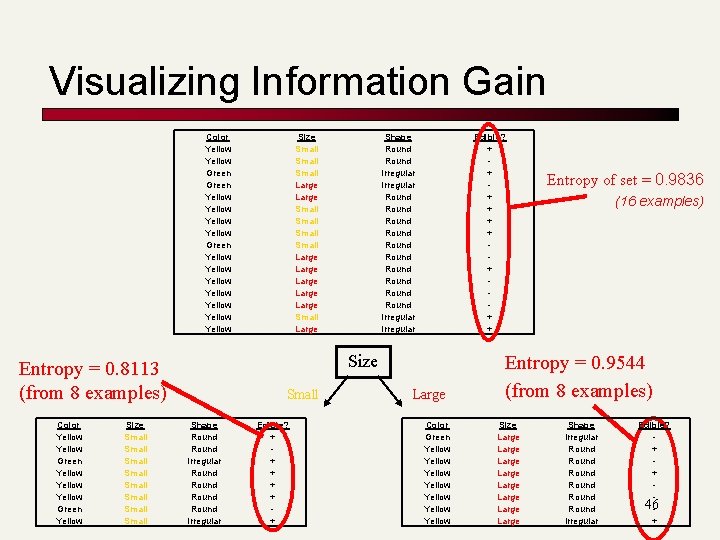
Visualizing Information Gain Color Yellow Green Yellow Yellow Yellow Size Small Small Shape Round Irregular Round Round Round Irregular Edible? + + + + + Size Entropy = 0. 8113 (from 8 examples) Color Yellow Green Yellow Size Small Small Large Large Small Shape Round Irregular Round Irregular Edible? + + + Large Color Green Yellow Yellow Entropy of set = 0. 9836 (16 examples) Entropy = 0. 9544 (from 8 examples) Size Large Large Shape Irregular Round Round Irregular Edible? + + 46+

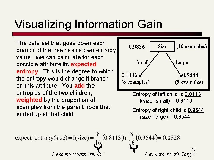
Visualizing Information Gain The data set that goes down each Size (16 examples) 0. 9836 branch of the tree has its own entropy value. We can calculate for each Small Large possible attribute its expected entropy. This is the degree to which 0. 8113 0. 9544 the entropy would change if branch (8 examples) on this attribute. You add the entropies of the two children, Entropy of left child is 0. 8113 weighted by the proportion of I(size=small) = 0. 8113 examples from the parent node that Entropy of right child is 0. 9544 ended up at that child. I(size=large) = 0. 9544 8 examples with ‘small’ 47 8 examples with ‘large’

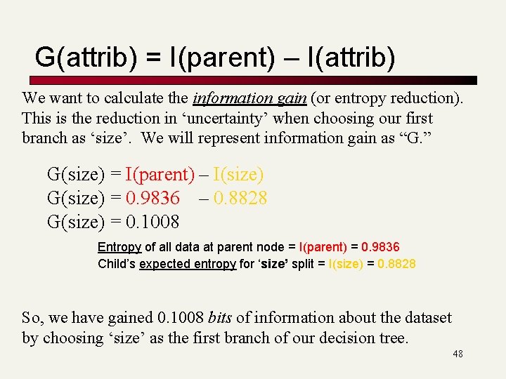
G(attrib) = I(parent) – I(attrib) We want to calculate the information gain (or entropy reduction). This is the reduction in ‘uncertainty’ when choosing our first branch as ‘size’. We will represent information gain as “G. ” G(size) = I(parent) – I(size) G(size) = 0. 9836 – 0. 8828 G(size) = 0. 1008 Entropy of all data at parent node = I(parent) = 0. 9836 Child’s expected entropy for ‘size’ split = I(size) = 0. 8828 So, we have gained 0. 1008 bits of information about the dataset by choosing ‘size’ as the first branch of our decision tree. 48

Decision Tree Learning n Fully grown trees tend to have decision rules that are overly specific and are therefore unable to categorize documents well n n Therefore, pruning or early stopping methods for Decision Trees are normally a standard part of classification packages Use of small number of features is potentially bad in text cat, but in practice decision trees do well for some text classification tasks Decision trees are very easily interpreted by humans – much more easily than probabilistic methods like Naive Bayes Decision Trees are normally regarded as a symbolic machine learning algorithm, though they can be used probabilistically 49

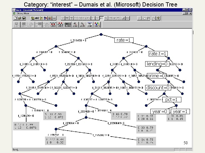
Category: “interest” – Dumais et al. (Microsoft) Decision Tree rate=1 rate. t=1 lending=0 prime=0 discount=0 pct=1 year=0 year=1 50

Summary: Representation of Text Categorization Attributes n n Representations of text are usually very high dimensional (one feature for each word) High-bias algorithms that prevent overfitting in high-dimensional space generally work best For most text categorization tasks, there are many relevant features and many irrelevant ones Methods that combine evidence from many or all features (e. g. naive Bayes, k. NN, neural-nets) often tend to work better than ones that try to isolate just a few relevant features (standard decision-tree or rule induction)* *Although one can compensate by using many rules 51