Vector Semantics Dense Vectors Dan Jurafsky Sparse versus

Vector Semantics Dense Vectors

Dan Jurafsky Sparse versus dense vectors • PPMI vectors are • long (length |V|= 20, 000 to 50, 000) • sparse (most elements are zero) • Alternative: learn vectors which are • short (length 200 -1000) • dense (most elements are non-zero) 2

Dan Jurafsky Sparse versus dense vectors • Why dense vectors? • Short vectors may be easier to use as features in machine learning (less weights to tune) • Dense vectors may generalize better than storing explicit counts • They may do better at capturing synonymy: • car and automobile are synonyms; but are represented as distinct dimensions; this fails to capture similarity between a word with car as a neighbor and a word with automobile as a neighbor 3

Dan Jurafsky Three methods for getting short dense vectors • Singular Value Decomposition (SVD) • A special case of this is called LSA – Latent Semantic Analysis • “Neural Language Model”-inspired predictive models • skip-grams and CBOW • Brown clustering 4

Vector Semantics Dense Vectors via SVD

Dan Jurafsky Intuition • Approximate an N-dimensional dataset using fewer dimensions • By first rotating the axes into a new space • In which the highest order dimension captures the most variance in the original dataset • And the next dimension captures the next most variance, etc. • Many such (related) methods: 6 • PCA – principle components analysis • Factor Analysis • SVD

Dan Jurafsky Dimensionality reduction 7

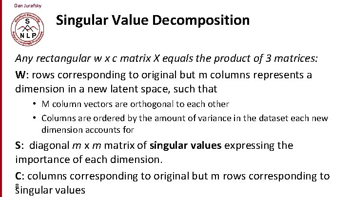
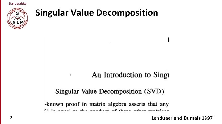
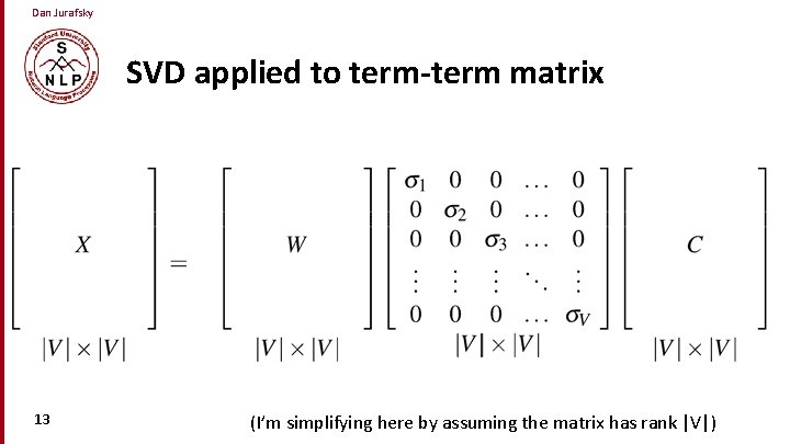
Dan Jurafsky Singular Value Decomposition Any rectangular w x c matrix X equals the product of 3 matrices: W: rows corresponding to original but m columns represents a dimension in a new latent space, such that • M column vectors are orthogonal to each other • Columns are ordered by the amount of variance in the dataset each new dimension accounts for S: diagonal m x m matrix of singular values expressing the importance of each dimension. C: columns corresponding to original but m rows corresponding to 8 singular values

Dan Jurafsky Singular Value Decomposition 9 Landuaer and Dumais 1997

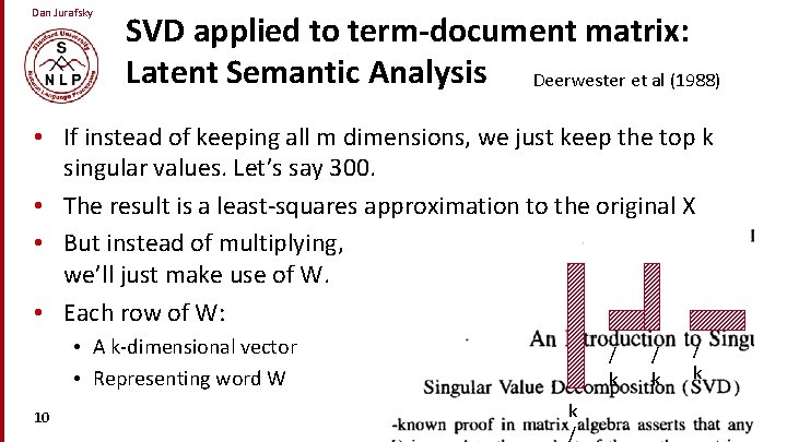
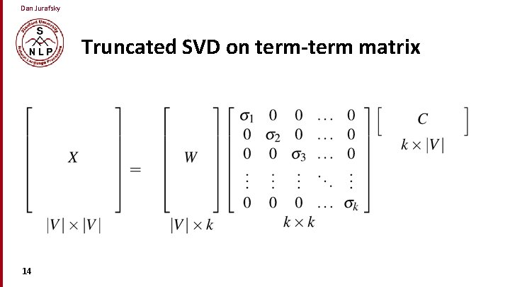
Dan Jurafsky SVD applied to term-document matrix: Latent Semantic Analysis Deerwester et al (1988) • If instead of keeping all m dimensions, we just keep the top k singular values. Let’s say 300. • The result is a least-squares approximation to the original X • But instead of multiplying, we’ll just make use of W. • Each row of W: • A k-dimensional vector • Representing word W 10 / k k / / k

Dan Jurafsky LSA more details • 300 dimensions are commonly used • The cells are commonly weighted by a product of two weights • Local weight: Log term frequency • Global weight: either idf or an entropy measure 11

Dan Jurafsky Let’s return to PPMI word-word matrices • Can we apply to SVD to them? 12

Dan Jurafsky SVD applied to term-term matrix 13 (I’m simplifying here by assuming the matrix has rank |V|)

Dan Jurafsky Truncated SVD on term-term matrix 14

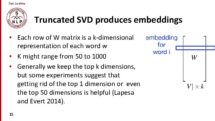
Dan Jurafsky Truncated SVD produces embeddings • Each row of W matrix is a k-dimensional representation of each word w • K might range from 50 to 1000 • Generally we keep the top k dimensions, but some experiments suggest that getting rid of the top 1 dimension or even the top 50 dimensions is helpful (Lapesa and Evert 2014). 15

Dan Jurafsky Embeddings versus sparse vectors • Dense SVD embeddings sometimes work better than sparse PPMI matrices at tasks like word similarity 16 • Denoising: low-order dimensions may represent unimportant information • Truncation may help the models generalize better to unseen data. • Having a smaller number of dimensions may make it easier for classifiers to properly weight the dimensions for the task. • Dense models may do better at capturing higher order cooccurrence.

Vector Semantics Embeddings inspired by neural language models: skip-grams and CBOW

Dan Jurafsky Prediction-based models: An alternative way to get dense vectors • Skip-gram (Mikolov et al. 2013 a) CBOW (Mikolov et al. 2013 b) • Learn embeddings as part of the process of word prediction. • Train a neural network to predict neighboring words • Inspired by neural net language models. • In so doing, learn dense embeddings for the words in the training corpus. • Advantages: 18 • Fast, easy to train (much faster than SVD) • Available online in the word 2 vec package • Including sets of pretrained embeddings!

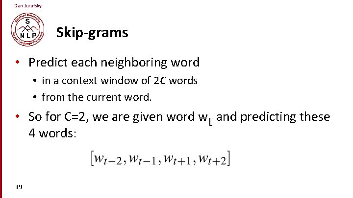
Dan Jurafsky Skip-grams • Predict each neighboring word • in a context window of 2 C words • from the current word. • So for C=2, we are given word wt and predicting these 4 words: 19

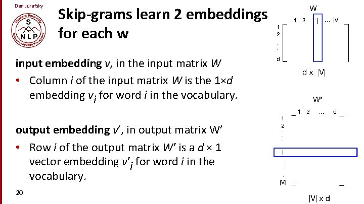
Dan Jurafsky Skip-grams learn 2 embeddings for each w input embedding v, in the input matrix W • Column i of the input matrix W is the 1×d embedding vi for word i in the vocabulary. output embedding v′, in output matrix W’ • Row i of the output matrix W′ is a d × 1 vector embedding v′i for word i in the vocabulary. 20

Dan Jurafsky Setup • Walking through corpus pointing at word w(t), whose index in the vocabulary is j, so we’ll call it wj (1 < j < |V |). • Let’s predict w(t+1) , whose index in the vocabulary is k (1 < k < |V |). Hence our task is to compute P(wk|wj). 21

Dan Jurafsky 22 Intuition: similarity as dot-product between a target vector and context vector

Dan Jurafsky Similarity is computed from dot product • Remember: two vectors are similar if they have a high dot product • Cosine is just a normalized dot product • So: • Similarity(j, k) ∝ ck ∙ vj • We’ll need to normalize to get a probability 23

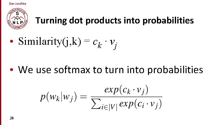
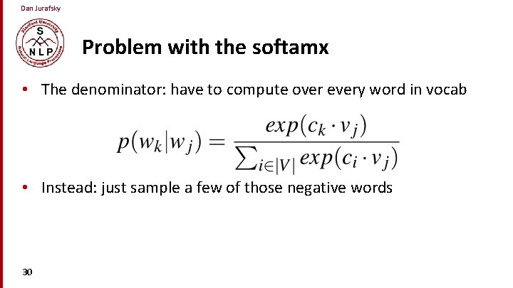
Dan Jurafsky Turning dot products into probabilities • Similarity(j, k) = ck ∙ vj • We use softmax to turn into probabilities 24

Dan Jurafsky Embeddings from W and W’ • Since we have two embeddings, vj and cj for each word wj • We can either: • Just use vj • Sum them • Concatenate them to make a double-length embedding 25

Dan Jurafsky Learning • Start with some initial embeddings (e. g. , random) • iteratively make the embeddings for a word • more like the embeddings of its neighbors • less like the embeddings of other words. 26

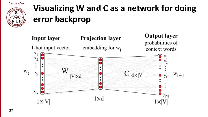
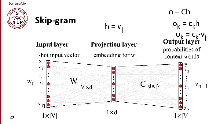
Dan Jurafsky 27 Visualizing W and C as a network for doing error backprop

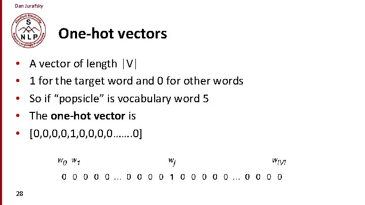
Dan Jurafsky One-hot vectors • • • 28 A vector of length |V| 1 for the target word and 0 for other words So if “popsicle” is vocabulary word 5 The one-hot vector is [0, 0, 1, 0, 0……. 0]

Dan Jurafsky Skip-gram 29 h = vj o = Ch ok = c k h ok = ck∙vj

Dan Jurafsky Problem with the softamx • The denominator: have to compute over every word in vocab • Instead: just sample a few of those negative words 30

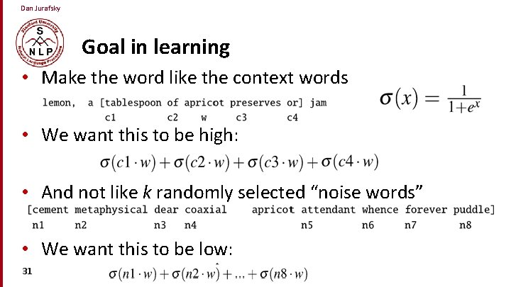
Dan Jurafsky Goal in learning • Make the word like the context words • We want this to be high: • And not like k randomly selected “noise words” • We want this to be low: 31

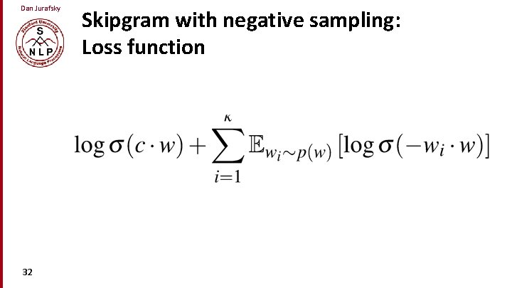
Dan Jurafsky 32 Skipgram with negative sampling: Loss function

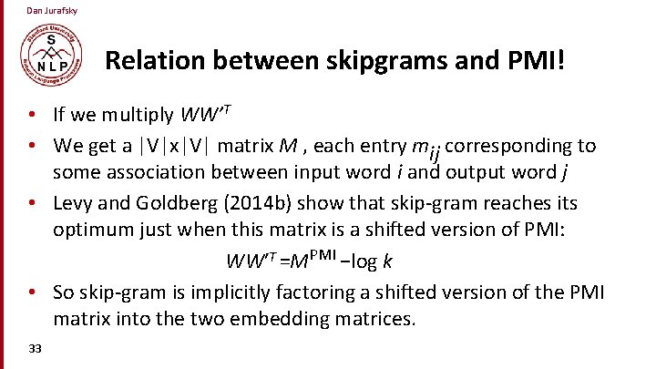
Dan Jurafsky Relation between skipgrams and PMI! • If we multiply WW’T • We get a |V|x|V| matrix M , each entry mij corresponding to some association between input word i and output word j • Levy and Goldberg (2014 b) show that skip-gram reaches its optimum just when this matrix is a shifted version of PMI: WW′T =MPMI −log k • So skip-gram is implicitly factoring a shifted version of the PMI matrix into the two embedding matrices. 33

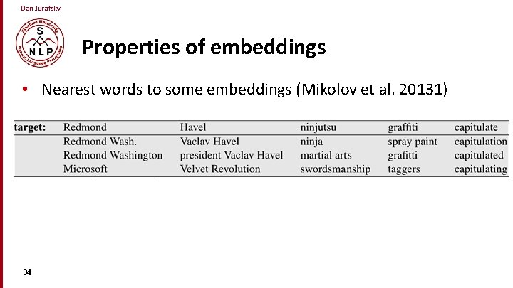
Dan Jurafsky Properties of embeddings • Nearest words to some embeddings (Mikolov et al. 20131) 34

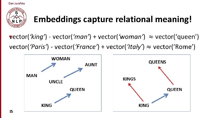
Dan Jurafsky Embeddings capture relational meaning! • 35

Vector Semantics Brown clustering

Dan Jurafsky Brown clustering • An agglomerative clustering algorithm that clusters words based on which words precede or follow them • These word clusters can be turned into a kind of vector • We’ll give a very brief sketch here. 37

Dan Jurafsky Brown clustering algorithm • Each word is initially assigned to its own cluster. • We now consider merging each pair of clusters. Highest quality merge is chosen. • Quality = merges two words that have similar probabilities of preceding and following words • (More technically quality = smallest decrease in the likelihood of the corpus according to a class-based language model) • Clustering proceeds until all words are in one big cluster. 38

Dan Jurafsky Brown Clusters as vectors • By tracing the order in which clusters are merged, the model builds a binary tree from bottom to top. • Each word represented by binary string = path from root to leaf • Each intermediate node is a cluster • Chairman is 0010, “months” = 01, and verbs = 1 39

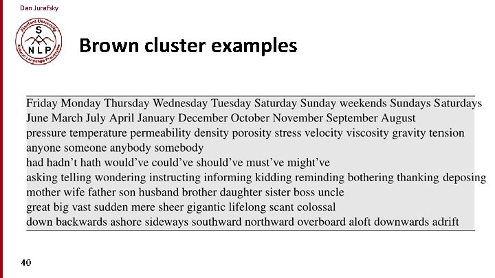
Dan Jurafsky Brown cluster examples 40

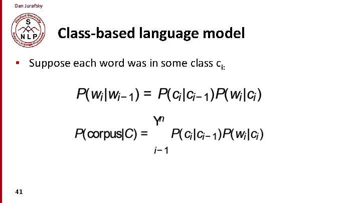
Dan Jurafsky Class-based language model • Suppose each word was in some class ci: 41