Vector Autoregression 1 Overview Vector Autoregression VAR model

Vector Autoregression 1

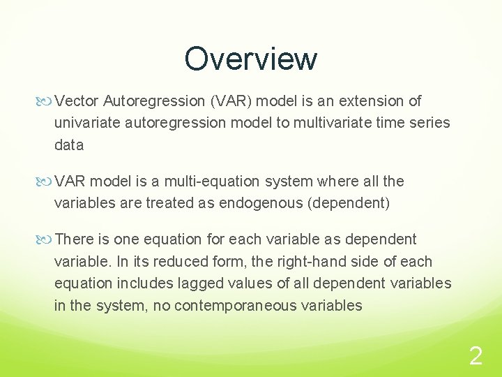
Overview Vector Autoregression (VAR) model is an extension of univariate autoregression model to multivariate time series data VAR model is a multi-equation system where all the variables are treated as endogenous (dependent) There is one equation for each variable as dependent variable. In its reduced form, the right-hand side of each equation includes lagged values of all dependent variables in the system, no contemporaneous variables 2

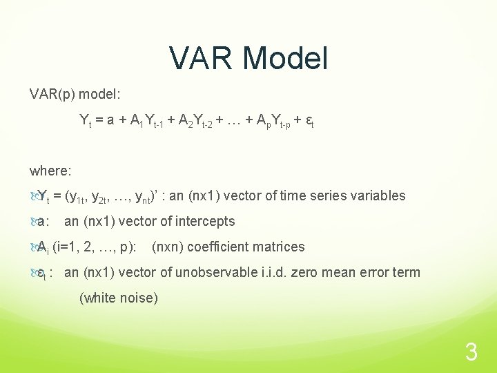
VAR Model VAR(p) model: Yt = a + A 1 Yt-1 + A 2 Yt-2 + … + Ap. Yt-p + εt where: Yt = (y 1 t, y 2 t, …, ynt)’ : an (nx 1) vector of time series variables a: an (nx 1) vector of intercepts Ai (i=1, 2, …, p): (nxn) coefficient matrices εt : an (nx 1) vector of unobservable i. i. d. zero mean error term (white noise) 3

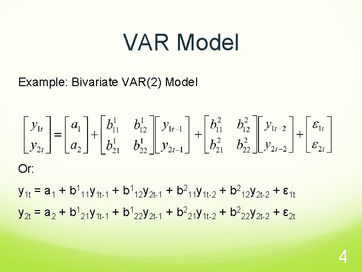
VAR Model Example: Bivariate VAR(2) Model Or: y 1 t = a 1 + b 111 y 1 t-1 + b 112 y 2 t-1 + b 211 y 1 t-2 + b 212 y 2 t-2 + ε 1 t y 2 t = a 2 + b 121 y 1 t-1 + b 122 y 2 t-1 + b 221 y 1 t-2 + b 222 y 2 t-2 + ε 2 t 4

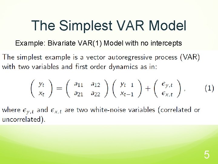
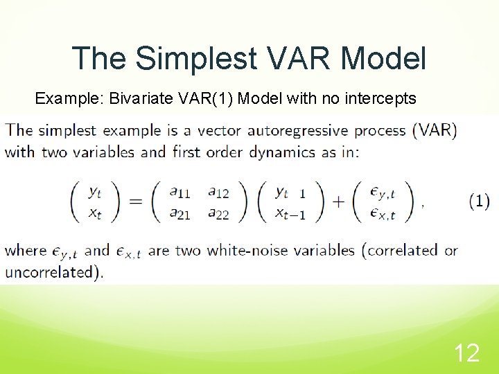
The Simplest VAR Model Example: Bivariate VAR(1) Model with no intercepts 5

The Marginal Models 6

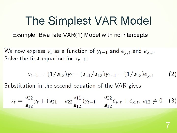
The Simplest VAR Model Example: Bivariate VAR(1) Model with no intercepts 7

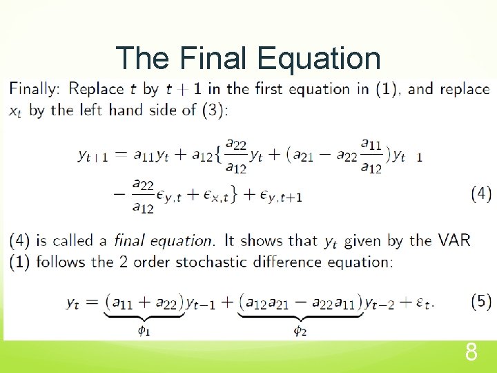
The Final Equation 8

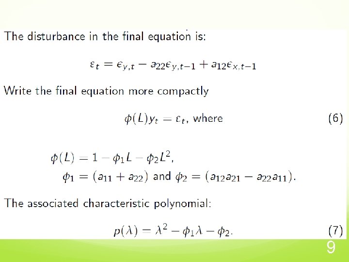
The Simplest VAR Model 9

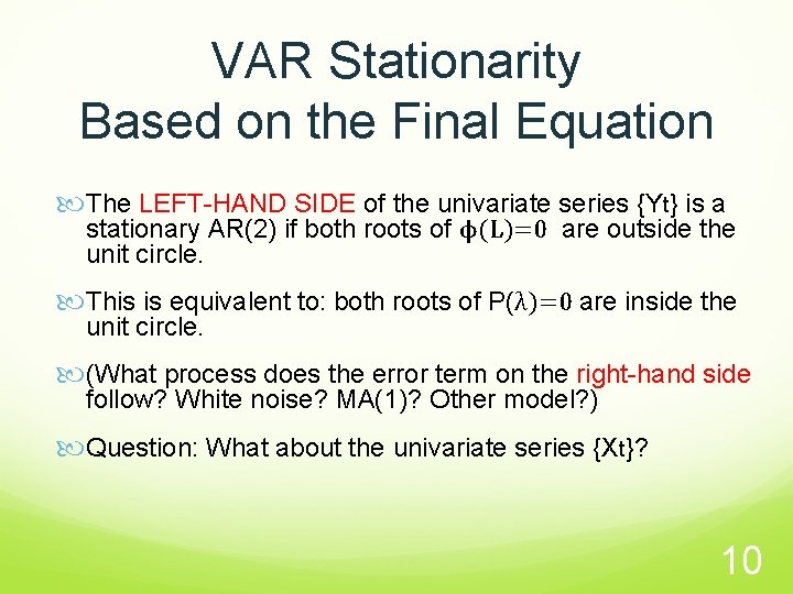
VAR Stationarity Based on the Final Equation The LEFT-HAND SIDE of the univariate series {Yt} is a stationary AR(2) if both roots of ϕ(L)=0 are outside the unit circle. This is equivalent to: both roots of P(λ)=0 are inside the unit circle. (What process does the error term on the right-hand side follow? White noise? MA(1)? Other model? ) Question: What about the univariate series {Xt}? 10

Check for Stationarity 11

The Simplest VAR Model Example: Bivariate VAR(1) Model with no intercepts 12

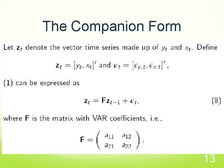
The Companion Form 13

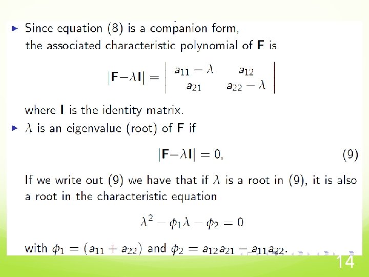
The Companion Form II 14

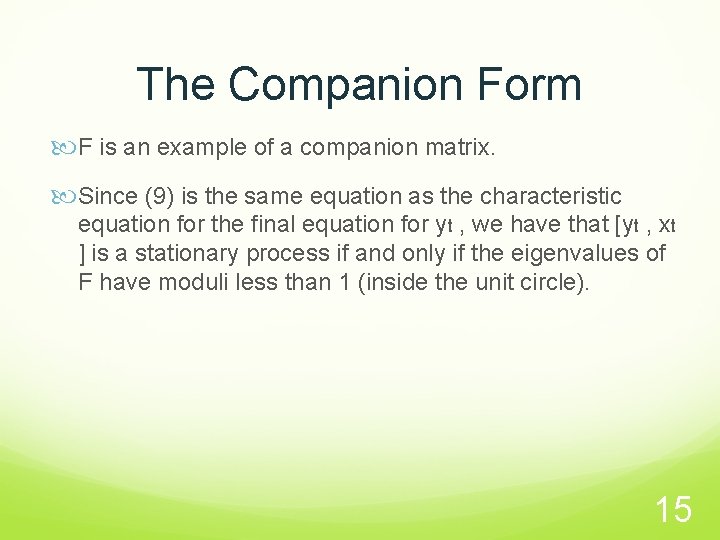
The Companion Form F is an example of a companion matrix. Since (9) is the same equation as the characteristic equation for the final equation for yt , we have that [yt , xt ] is a stationary process if and only if the eigenvalues of F have moduli less than 1 (inside the unit circle). 15

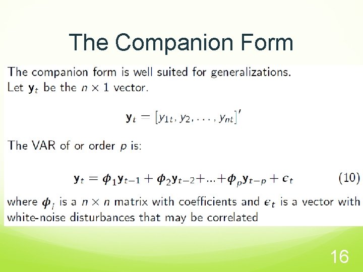
The Companion Form 16

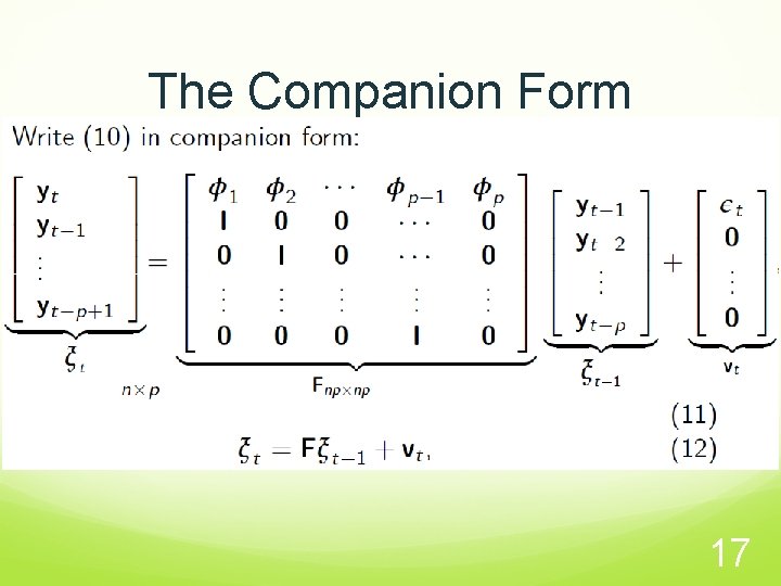
The Companion Form 17

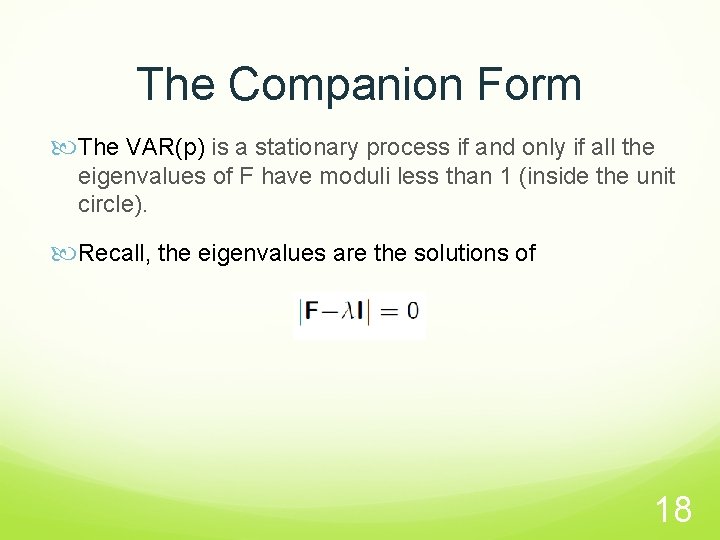
The Companion Form The VAR(p) is a stationary process if and only if all the eigenvalues of F have moduli less than 1 (inside the unit circle). Recall, the eigenvalues are the solutions of 18

Why do we need VAR? Time-series data with autoregressive in nature (serially correlated) VAR model is one of the most successful and flexible models for the analysis of multivariate time series Especially useful for describing the dynamic behavior of economic and financial time series Useful forecasting 19

Applications of VAR Analysis of system response to different shocks/impacts Model-based forecast. In general VAR encompasses correlation information of the observed data and use this correlation information to forecast future movements or changes of the variable of interest 20

Applications of VAR In economics, VAR is used to forecast macroeconomic variables, such as GDP, money supply, and unemployment In finance, predict spot prices and future prices of securities; foreign exchange rates across markets 21

Applications of VAR In accounting, predict different accounting variables such as sales, earnings, and accruals In marketing, VAR can be used to evaluate the impact of different factors on consumer behavior and forecast its future change. 22

Forecasting 23

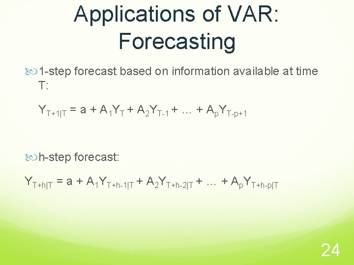
Applications of VAR: Forecasting 1 -step forecast based on information available at time T: YT+1|T = a + A 1 YT + A 2 YT-1 + … + Ap. YT-p+1 h-step forecast: YT+h|T = a + A 1 YT+h-1|T + A 2 YT+h-2|T + … + Ap. YT+h-p|T 24

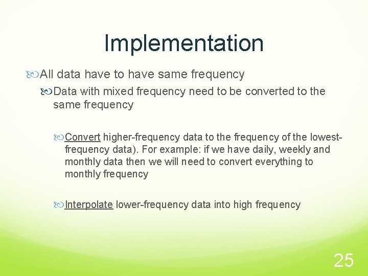
Implementation All data have to have same frequency Data with mixed frequency need to be converted to the same frequency Convert higher-frequency data to the frequency of the lowestfrequency data). For example: if we have daily, weekly and monthly data then we will need to convert everything to monthly frequency Interpolate lower-frequency data into high frequency 25

SAS & R for VAR 26

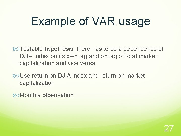
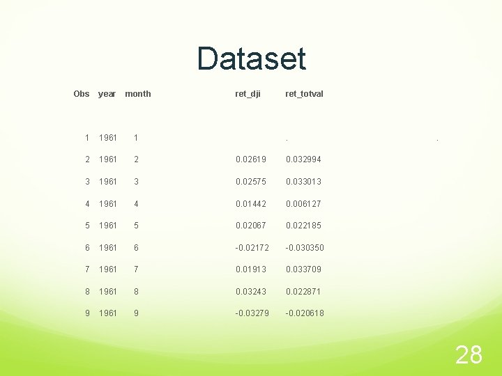
Example of VAR usage Testable hypothesis: there has to be a dependence of DJIA index on its own lag and on lag of total market capitalization and vice versa Use return on DJIA index and return on market capitalization Monthly observation 27

Dataset Obs year month ret_dji ret_totval 1 1961 1 . 2 1961 2 0. 02619 0. 032994 3 1961 3 0. 02575 0. 033013 4 1961 4 0. 01442 0. 006127 5 1961 5 0. 02067 0. 022185 6 1961 6 -0. 02172 -0. 030350 7 1961 7 0. 01913 0. 033709 8 1961 8 0. 03243 0. 022871 9 1961 9 -0. 03279 -0. 020618 . 28

SAS 29

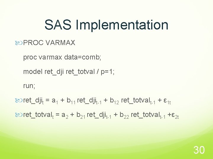
SAS Implementation PROC VARMAX proc varmax data=comb; model ret_dji ret_totval / p=1; run; ret_djit = a 1 + b 11 ret_djit-1 + b 12 ret_totvalt-1 + ε 1 t ret_totvalt = a 2 + b 21 ret_djit-1 + b 22 ret_totvalt-1 +ε 2 t 30

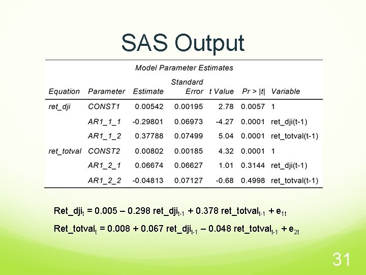
SAS Output Ret_djit = 0. 005 – 0. 298 ret_djit-1 + 0. 378 ret_totvalt-1 + e 1 t Ret_totvalt = 0. 008 + 0. 067 ret_djit-1 – 0. 048 ret_totvalt-1 + e 2 t 31

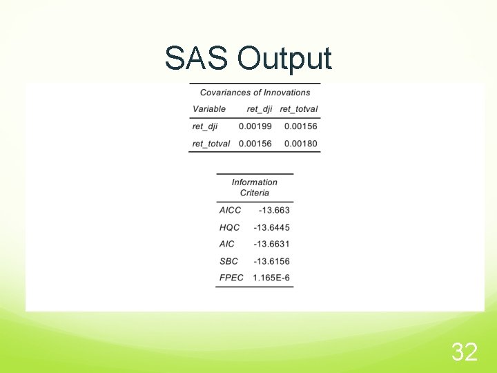
SAS Output 32

R 33

R for VARs are implemented in the vars package in R. It contains a function VARselect to choose the number of lags p using four different information criteria: AIC, HQ, SC and FPE. We have met the AIC before, and SC is simply another name for the BIC (SC stands for Schwarz Criterion after Gideon Schwarz who proposed it). HQ is the Hannan-Quinn criterion and FPE is the “Final Prediction Error” criterion. Care should be taken using the AIC as it tends to choose large numbers of lags. Instead, for VAR models, we prefer to use the BIC. 34

Concerns Assuming all variables are endogenous If time-series data are nonstationary (containing stochastic trends), while it is possible to estimate VAR in levels, it is preferable to estimate VAR in first differences Uncertainty about number of lags (using LR test, Information criteria: AIC, BIC etc. ) 35

Concerns Data requirements (long time series) Imprecise estimated coefficients (overfitting the model). Solution – restrict or weight coefficients Computationally intensive 36

References courses. ttu. edu/isqs 6348 westfall/VARPresentation. ppt Chapter 1: Vector Autoregressions. https: //www 2. bc. edu/~iacoviel/teach/0809/EC 751_files/ var. pdf Chapter 6: Multivariate time series models. www. nek. lu. se/. . . /Ch 6%20 Multivariate%20 time%20 seri es%20 models 37

References http: //www. uio. no/studier/emner/sv/oekonomi/ECON 51 01/v 11/undervisningsmateriale/Lect 7 v 11. pdf Dwyer, Gerald P. , Jr. Why Are Vector Autoregressions Useful in Finance? http: //jerrydwyer. com/pdf/lectvar. pdf Vector Autoregressions: Forecasting and Reality. http: //www. frbatlanta. org/filelegacydocs/robtallm an. pdf 38

References Chapter 11: Vector Autoregressive Models for Multivariate Time Series. http: //faculty. washington. edu/ezivot/econ 584/notes/var Models. pdf https: //www. otexts. org/fpp/9/2 39