Variance Component Estimation a k a NonSphericity Correction

Variance Component Estimation a. k. a. Non-Sphericity Correction

Overview • • Variance-Covariance Matrix What is (and isn’t) sphericity? Why is non-sphericity a problem? How do proper statisticians solve it? How did SPM 99 solve it. How does SPM 2 solve it? What is all the fuss? Some 2 nd level examples.

Variance-Covariance matrix Length of Swedish men Weight of Swedish men μ=180 cm, σ=14 cm (σ2=200) μ=80 kg, σ=14 kg (σ2=200) Each completely characterised by μ (mean) and σ2 (variance), i. e. we can calculate p(l|μ, σ2) for any l

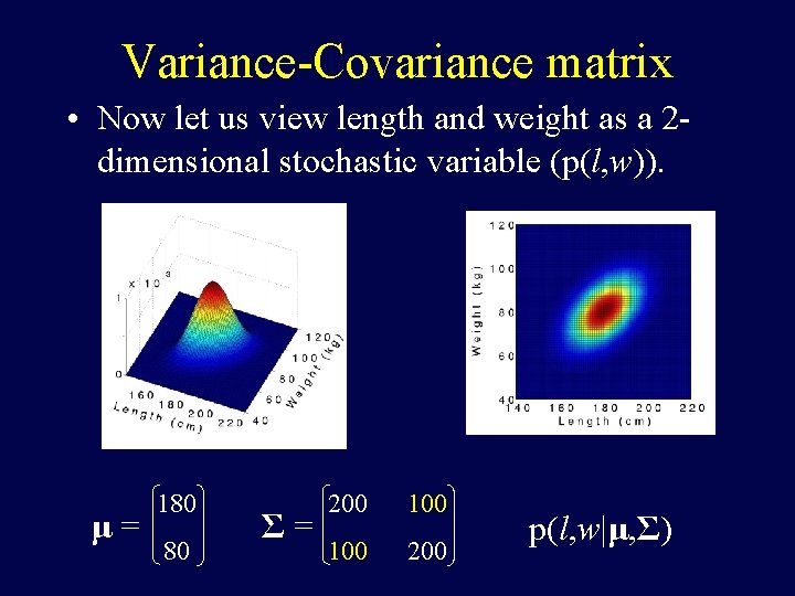
Variance-Covariance matrix • Now let us view length and weight as a 2 dimensional stochastic variable (p(l, w)). μ= 180 80 Σ= 200 100 200 p(l, w|μ, Σ)

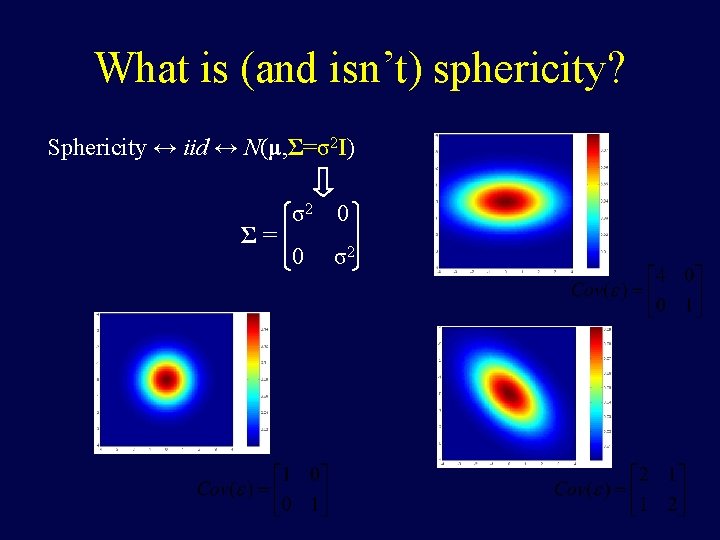
What is (and isn’t) sphericity? Sphericity ↔ iid ↔ N(μ, Σ=σ2 I) Σ= σ2 0 0 σ2

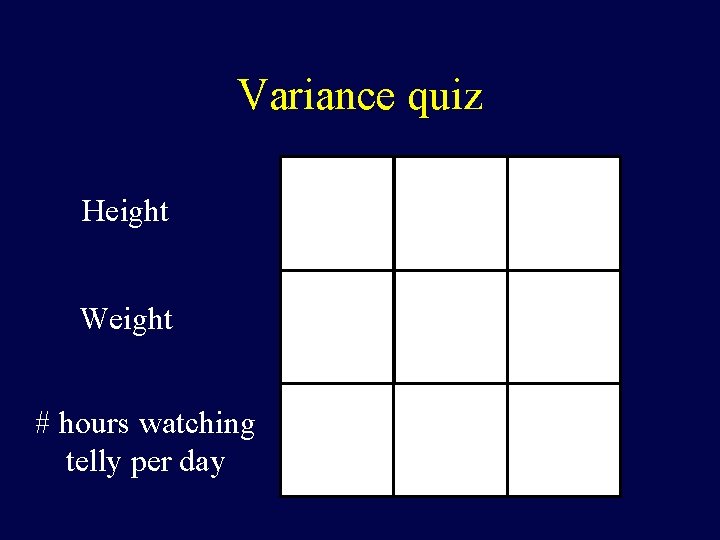
Variance quiz Height Weight # hours watching telly per day

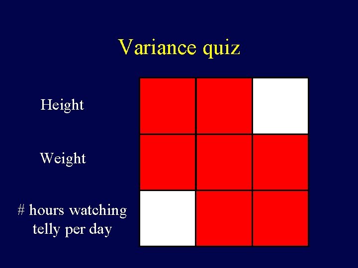
Variance quiz Height Weight # hours watching telly per day

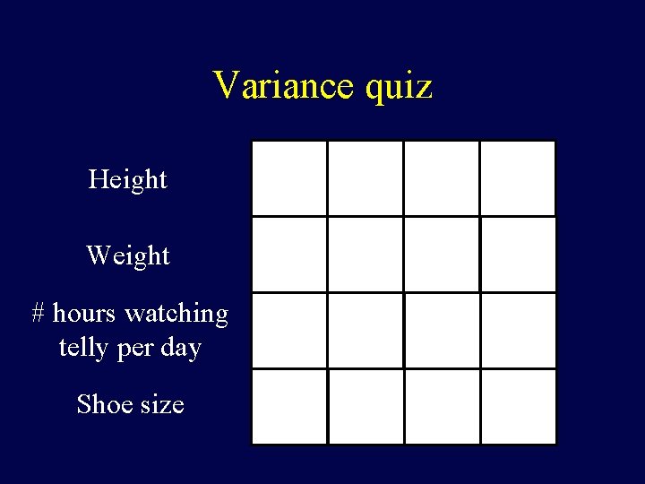
Variance quiz Height Weight # hours watching telly per day Shoe size

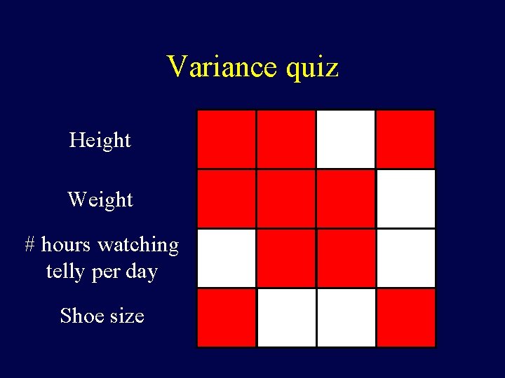
Variance quiz Height Weight # hours watching telly per day Shoe size

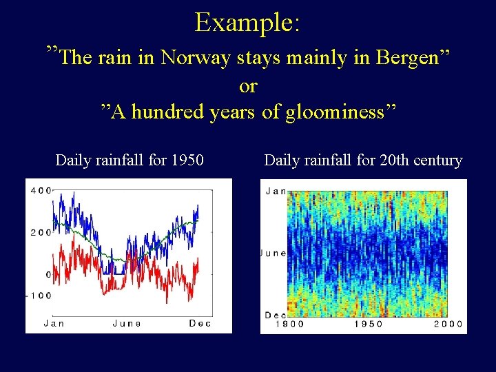
Example: ”The rain in Norway stays mainly in Bergen” or ”A hundred years of gloominess” Daily rainfall for 1950 Daily rainfall for 20 th century

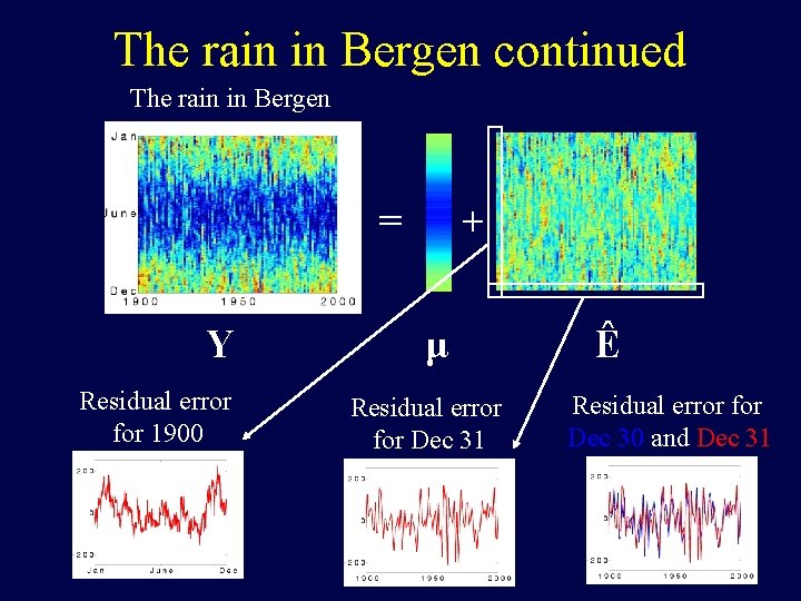
The rain in Bergen continued The rain in Bergen = Y Residual error for 1900 + μ Residual error for Dec 31 Ê Residual error for Dec 30 and Dec 31

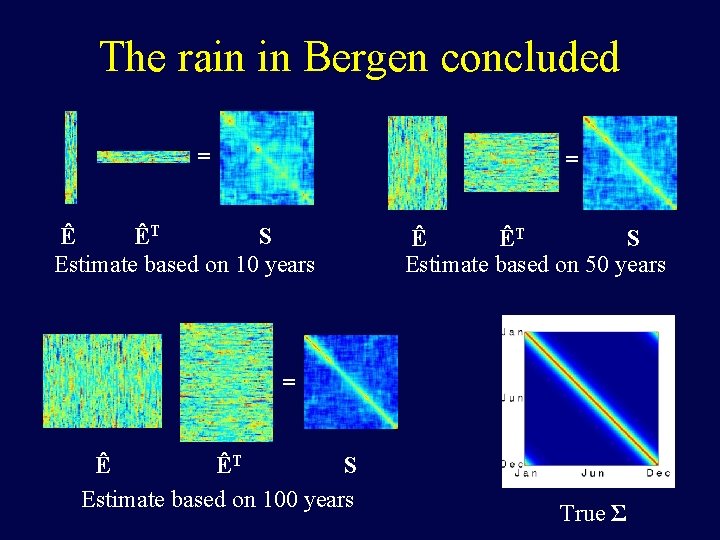
The rain in Bergen concluded = = Ê ÊT S Estimate based on 10 years Ê ÊT S Estimate based on 50 years = Ê ÊT S Estimate based on 100 years True Σ

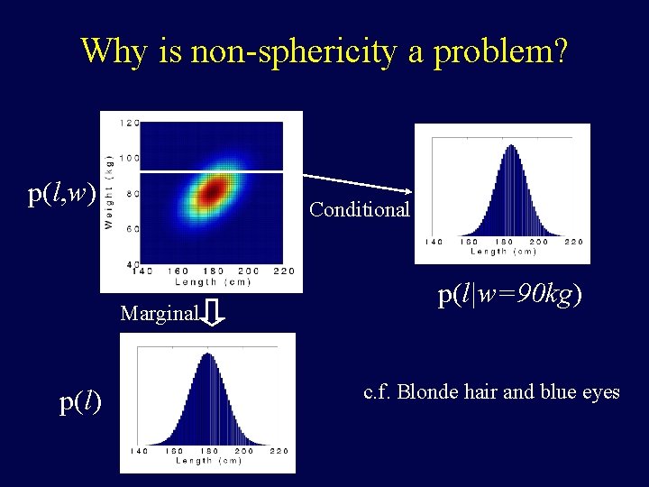
Why is non-sphericity a problem? p(l, w) Conditional Marginal p(l) p(l|w=90 kg) c. f. Blonde hair and blue eyes

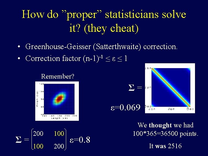
How do ”proper” statisticians solve it? (they cheat) • Greenhouse-Geisser (Satterthwaite) correction. • Correction factor (n-1)-1 ≤ ε ≤ 1 Remember? Σ= ε=0. 069 Σ= 200 100 200 ε=0. 8 We thought we had 100*365=36500 points. It was 2516

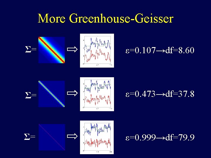
More Greenhouse-Geisser Σ= ε=0. 107→df=8. 60 Σ= ε=0. 473→df=37. 8 Σ= ε=0. 999→df=79. 9

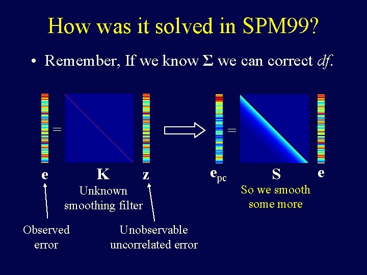
How was it solved in SPM 99? • Remember, If we know Σ we can correct df. = = e K z Unknown smoothing filter Observed error Unobservable uncorrelated error epc S So we smooth some more e

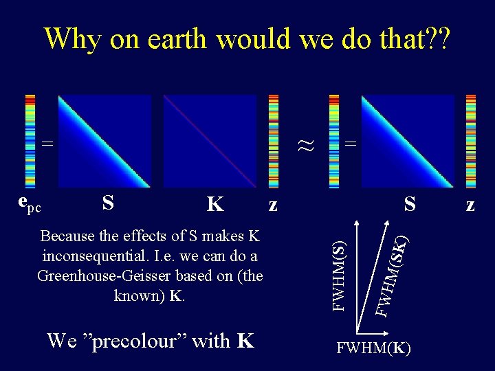
Why on earth would we do that? ? ≈ = We ”precolour” with K S ) Because the effects of S makes K inconsequential. I. e. we can do a Greenhouse-Geisser based on (the known) K. z M(SK K FWH S FWHM(S) epc = FWHM(K) z

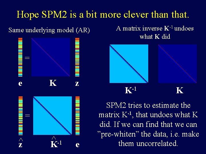
Hope SPM 2 is a bit more clever than that. Same underlying model (AR) A matrix inverse K-1 undoes what K did = e K z = ^z ^ -1 K e K-1 K SPM 2 tries to estimate the matrix K-1, that undoes what K did. If we can find that we can ”pre-whiten” the data, i. e. make them uncorrelated.

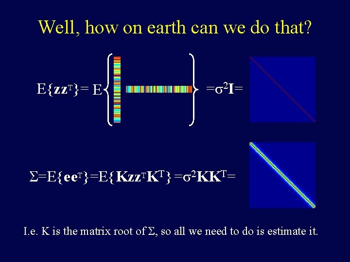
Well, how on earth can we do that? E{zz. T}= E =σ2 I= Σ=E{ee. T}=E{Kzz. TKT} =σ2 KKT= I. e. K is the matrix root of Σ, so all we need to do is estimate it.

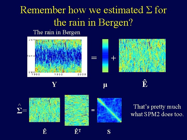
Remember how we estimated Σ for the rain in Bergen? The rain in Bergen = Y + Ê μ ^ Σ= That’s pretty much what SPM 2 does too. = Ê ÊT S

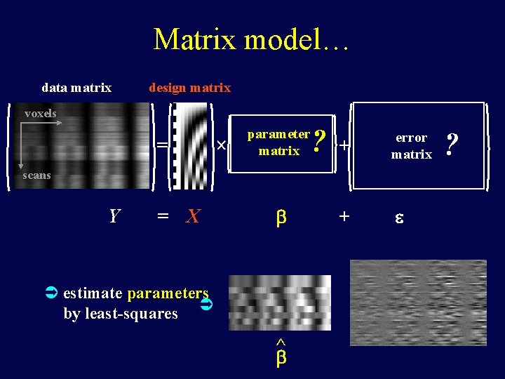
Matrix model… data matrix design matrix voxels = ? parameter matrix + error matrix + scans Y = X estimate parameters by least-squares ^ ?

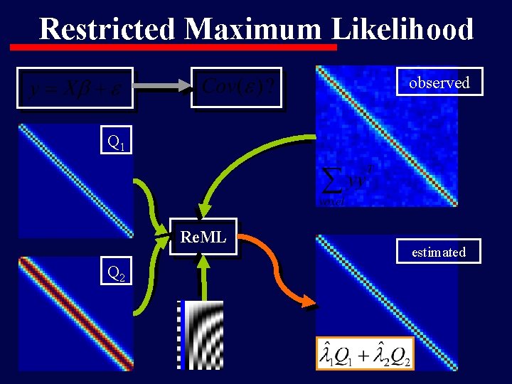
Restricted Maximum Likelihood observed Q 1 Re. ML Q 2 estimated

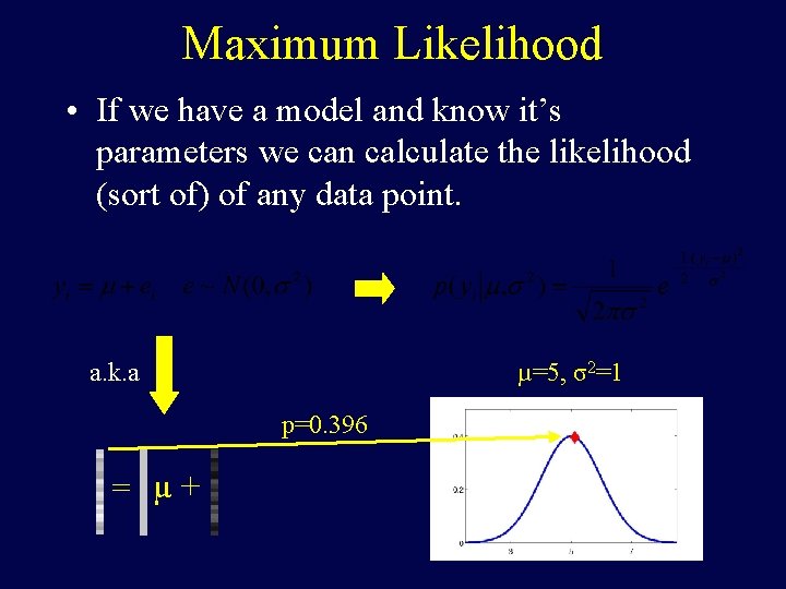
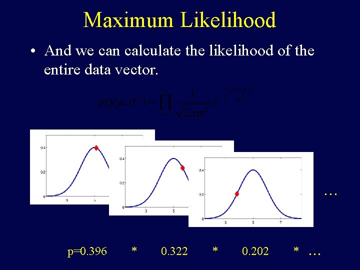
Maximum Likelihood • If we have a model and know it’s parameters we can calculate the likelihood (sort of) of any data point. a. k. a µ=5, σ2=1 p=0. 396 = µ+

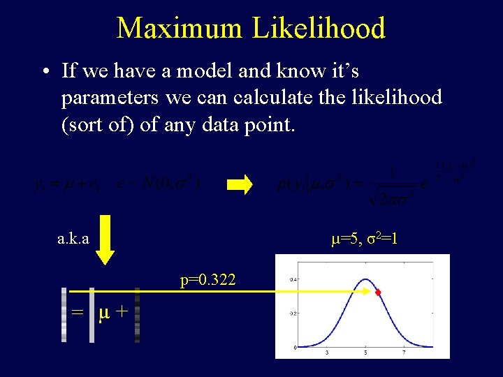
Maximum Likelihood • If we have a model and know it’s parameters we can calculate the likelihood (sort of) of any data point. a. k. a µ=5, σ2=1 p=0. 322 = µ+

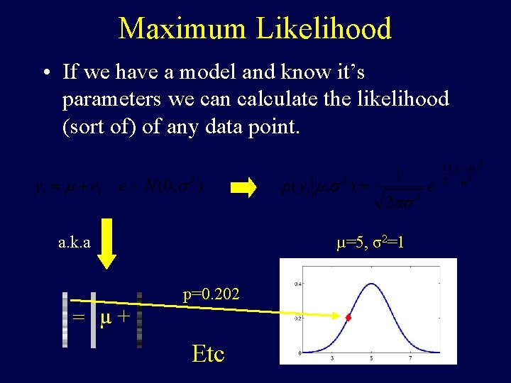
Maximum Likelihood • If we have a model and know it’s parameters we can calculate the likelihood (sort of) of any data point. a. k. a µ=5, σ2=1 p=0. 202 = µ+ Etc

Maximum Likelihood • And we can calculate the likelihood of the entire data vector. . p=0. 396 * 0. 322 * 0. 202 * . . .

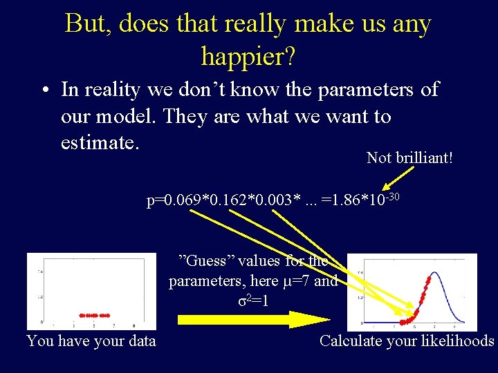
But, does that really make us any happier? • In reality we don’t know the parameters of our model. They are what we want to estimate. Not brilliant! p=0. 069*0. 162*0. 003*. . . =1. 86*10 -30 ”Guess” values for the parameters, here µ=7 and σ2=1 You have your data Calculate your likelihoods

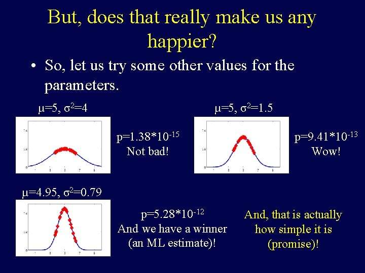
But, does that really make us any happier? • So, let us try some other values for the parameters. µ=5, σ2=4 µ=5, σ2=1. 5 p=1. 38*10 -15 Not bad! p=9. 41*10 -13 Wow! µ=4. 95, σ2=0. 79 p=5. 28*10 -12 And we have a winner (an ML estimate)! And, that is actually how simple it is (promise)!

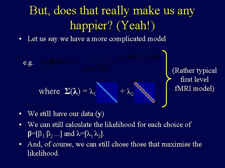
But, does that really make us any happier? (Yeah!) • Let us say we have a more complicated model e. g. where Σ(λ) = λ 1 + λ 2 (Rather typical first level f. MRI model) • We still have our data (y) • We can still calculate the likelihood for each choice of β=[β 1 β 2. . . ] and λ=[λ 1 λ 2]. • And, of course, we can still chose that maximise the likelihood.

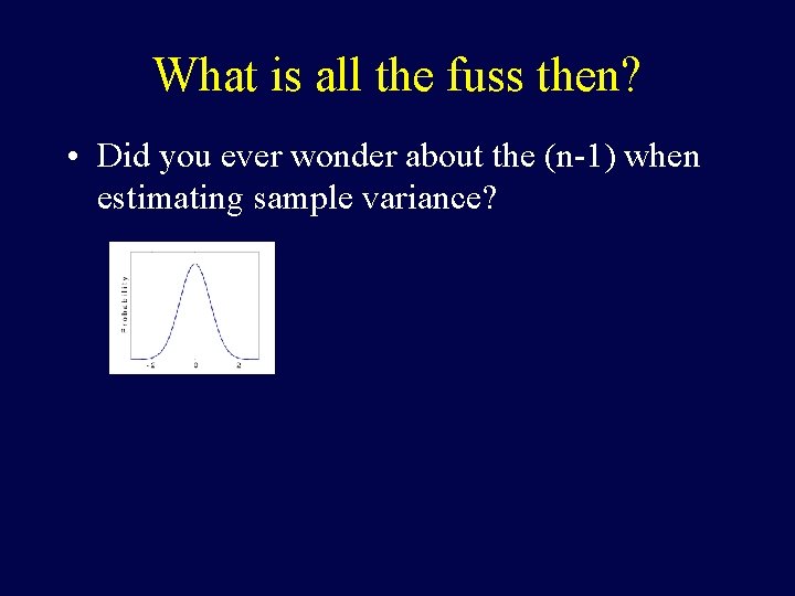
What is all the fuss then? • Did you ever wonder about the (n-1) when estimating sample variance?

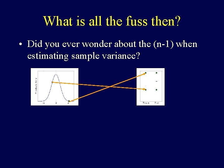
What is all the fuss then? • Did you ever wonder about the (n-1) when estimating sample variance?

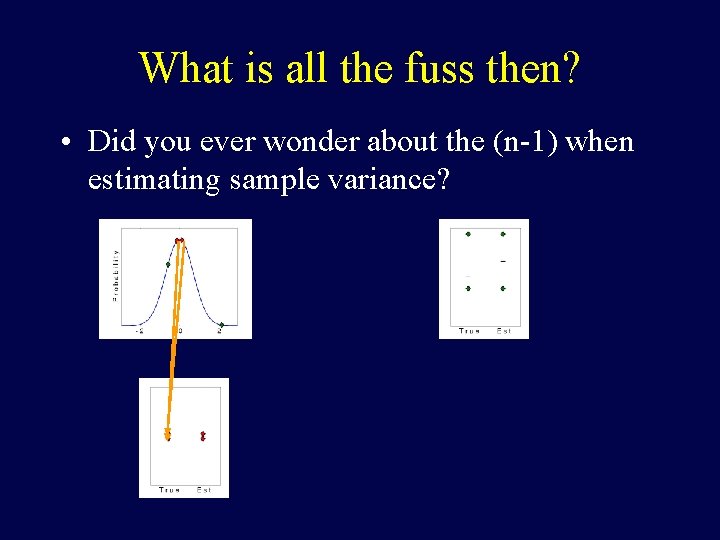
What is all the fuss then? • Did you ever wonder about the (n-1) when estimating sample variance?

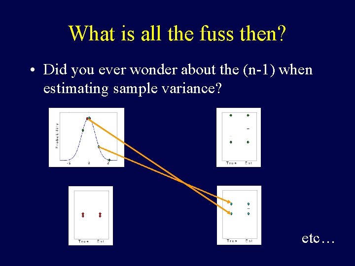
What is all the fuss then? • Did you ever wonder about the (n-1) when estimating sample variance? etc…

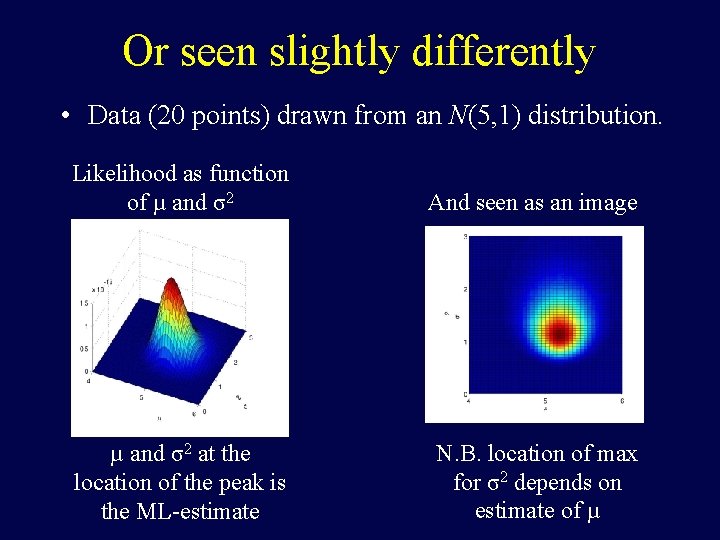
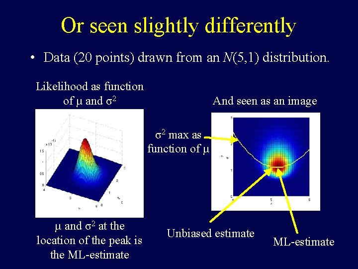
Or seen slightly differently • Data (20 points) drawn from an N(5, 1) distribution. Likelihood as function of µ and σ2 And seen as an image µ and σ2 at the location of the peak is the ML-estimate N. B. location of max for σ2 depends on estimate of µ

Or seen slightly differently • Data (20 points) drawn from an N(5, 1) distribution. Likelihood as function of µ and σ2 And seen as an image σ2 max as function of µ µ and σ2 at the location of the peak is the ML-estimate Unbiased estimate ML-estimate

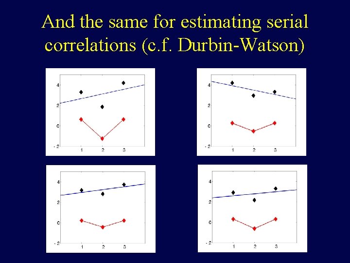
And the same for estimating serial correlations (c. f. Durbin-Watson)

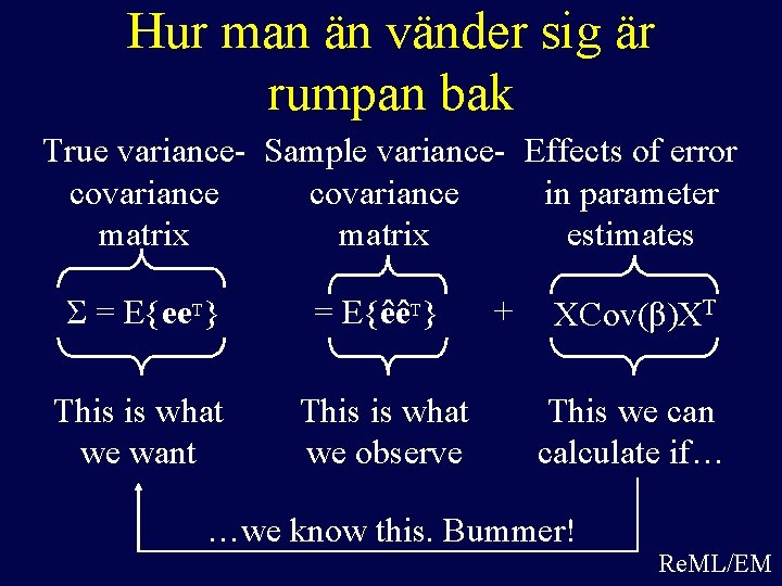
Hur man än vänder sig är rumpan bak True variance- Sample variance- Effects of error covariance in parameter matrix estimates Σ = E{ee. T} = E{êêT} This is what we want This is what we observe + XCov(β)XT This we can calculate if… …we know this. Bummer! Re. ML/EM

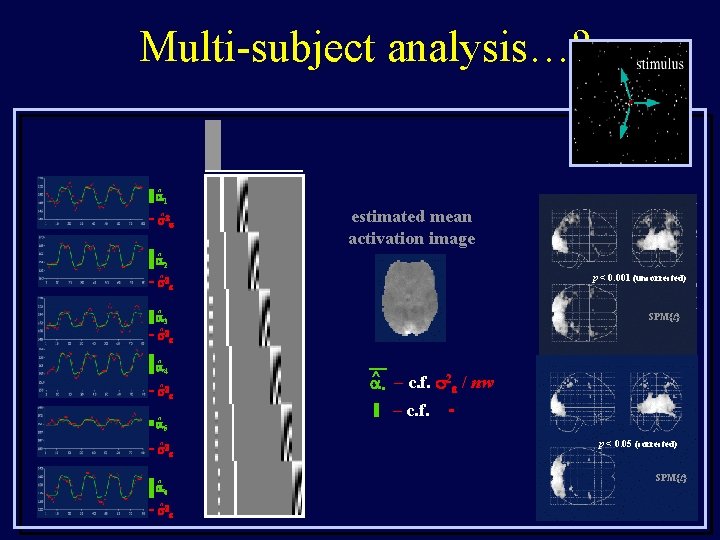
Multi-subject analysis…? ^ 1 ^ estimated mean activation image ^ 2 p < 0. 001 (uncorrected) ^ ^ 3 SPM{t} ^ ^ 4 ^ ^ 5 ^ ^ 6 ^ — ^ – c. f. 2 / nw • – c. f. p < 0. 05 (corrected) SPM{t}

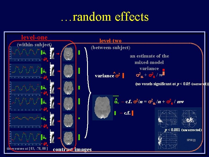
…random effects level-one level-two (within-subject) ^ 1 (between-subject) ^ ^ 2 ^ ^ 3 (no voxels significant at p < 0. 05 (corrected)) ^ ^ 4 variance^ 2 an estimate of the mixed-model variance 2 + 2 / w — ^ ^ – c. f. 2/n = 2 /n + 2 / nw • – c. f. ^ 5 ^ ^ 6 ^ timecourses at [ 03, -78, 00 ] p < 0. 001 (uncorrected) contrast images SPM{t}

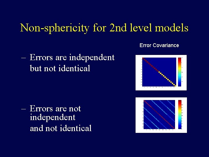
Non-sphericity for 2 nd level models Error Covariance – Errors are independent but not identical – Errors are not independent and not identical

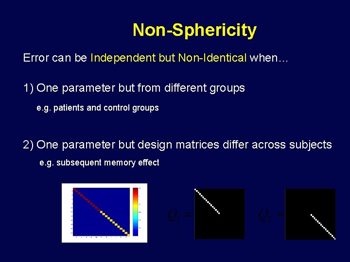
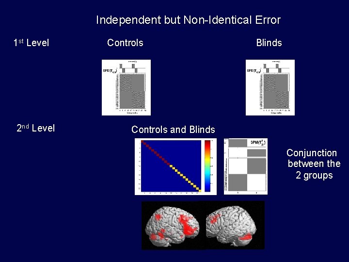
Non-Sphericity Error can be Independent but Non-Identical when… 1) One parameter but from different groups e. g. patients and control groups 2) One parameter but design matrices differ across subjects e. g. subsequent memory effect

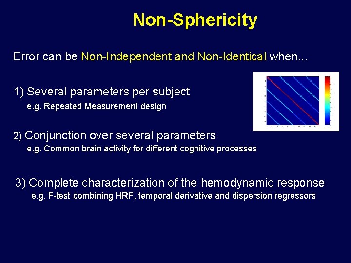
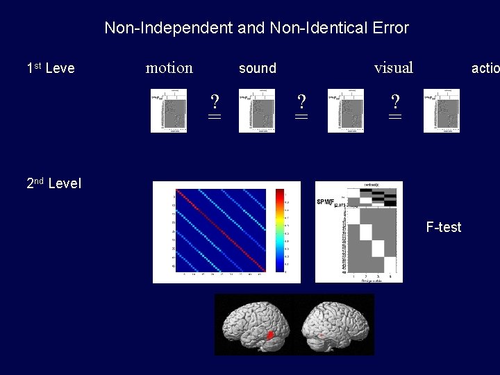
Non-Sphericity Error can be Non-Independent and Non-Identical when… 1) Several parameters per subject e. g. Repeated Measurement design 2) Conjunction over several parameters e. g. Common brain activity for different cognitive processes 3) Complete characterization of the hemodynamic response e. g. F-test combining HRF, temporal derivative and dispersion regressors

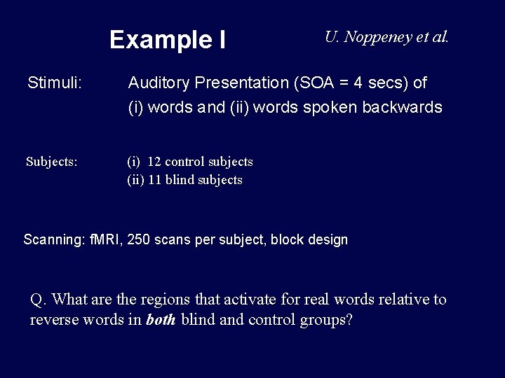
Example I U. Noppeney et al. Stimuli: Auditory Presentation (SOA = 4 secs) of (i) words and (ii) words spoken backwards Subjects: (i) 12 control subjects (ii) 11 blind subjects Scanning: f. MRI, 250 scans per subject, block design Q. What are the regions that activate for real words relative to reverse words in both blind and control groups?

Independent but Non-Identical Error 1 st Level 2 nd Level Controls Blinds Controls and Blinds Conjunction between the 2 groups

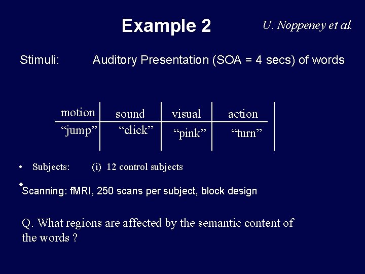
Example 2 Stimuli: U. Noppeney et al. Auditory Presentation (SOA = 4 secs) of words motion “jump” • Subjects: sound “click” visual action “pink” “turn” (i) 12 control subjects • Scanning: f. MRI, 250 scans per subject, block design Q. What regions are affected by the semantic content of the words ?

Non-Independent and Non-Identical Error 1 st Leve motion visual sound ? = actio ? = 2 nd Level F-test