Variance and Hypothesis Tests Econ 201 Econ Data

Variance and Hypothesis Tests Econ. 201 – Econ. Data Analysis

Difference in Means - Design • Try to isolate the experimental and control groups from each other while the experiment is conducted • Amounts to ensuring either that both groups are random samples drawn from the “universe” of such populations or that each group has equivalent values of any variable that might also (in addition to the experiment) alter its outcome

Example • “Men have higher cholesterol than women” • Want to isolate gender as a cause for cholesterol levels to vary. Yet we know many other things effect cholesterol – 2 are diet and genetics • Could isolate gender in two ways – 1: Draw random sample from the population • Ask, is cm>cw? – 2: Draw samples of men and women from populations with similar diets and genetics --- say 20 yr. old college students • Pose the same question as #1

Example, contd. • The Data in the example take the latter approach • Then pose the question formally as: – Ho: cm=cw (The null hypothesis) • that which you hope to disprove – H 1: cm≠cw (The alternative hypothesis)

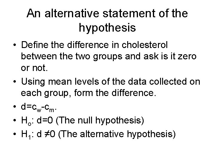
An alternative statement of the hypothesis • Define the difference in cholesterol between the two groups and ask is it zero or not. • Using mean levels of the data collected on each group, form the difference. • d=cw-cm. • Ho: d=0 (The null hypothesis) • H 1: d ≠ 0 (The alternative hypothesis)

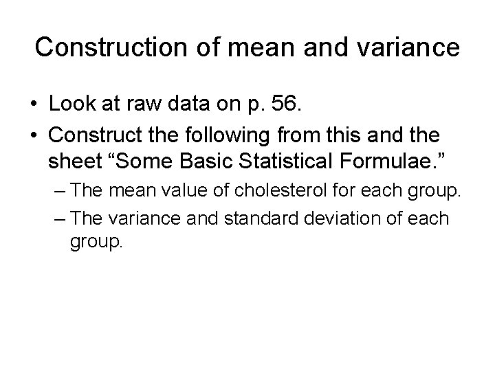
Construction of mean and variance • Look at raw data on p. 56. • Construct the following from this and the sheet “Some Basic Statistical Formulae. ” – The mean value of cholesterol for each group. – The variance and standard deviation of each group.

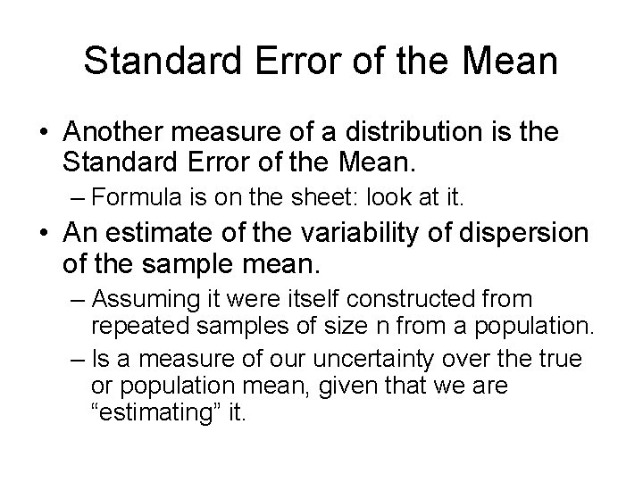
Standard Error of the Mean • Another measure of a distribution is the Standard Error of the Mean. – Formula is on the sheet: look at it. • An estimate of the variability of dispersion of the sample mean. – Assuming it were itself constructed from repeated samples of size n from a population. – Is a measure of our uncertainty over the true or population mean, given that we are “estimating” it.

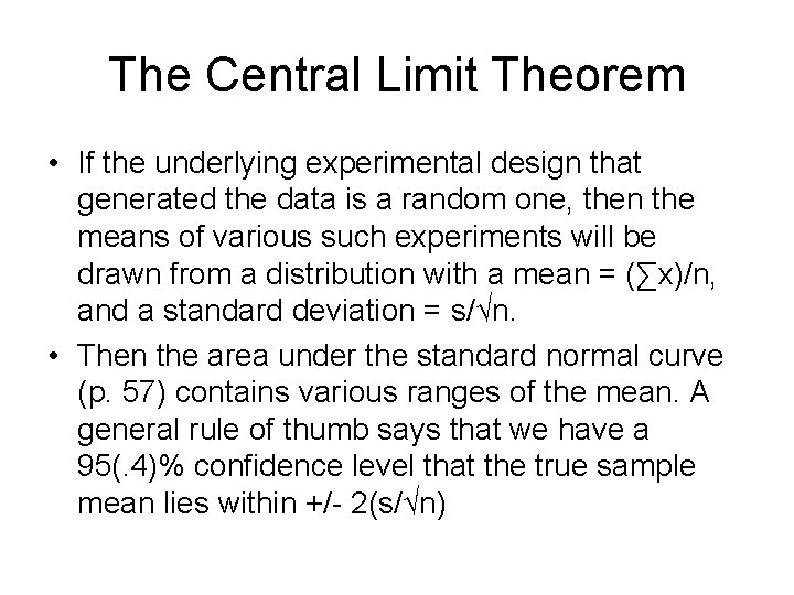
The Central Limit Theorem • If the underlying experimental design that generated the data is a random one, then the means of various such experiments will be drawn from a distribution with a mean = (∑x)/n, and a standard deviation = s/√n. • Then the area under the standard normal curve (p. 57) contains various ranges of the mean. A general rule of thumb says that we have a 95(. 4)% confidence level that the true sample mean lies within +/- 2(s/√n)

Intuition • Calculate the interval around each group’s mean with the standard errors of the means (see page 57). • The further apart are the means and the smaller the dispersions around these means (stnd. errors), the more likely we are to determine that the mean levels of the two groups are different.

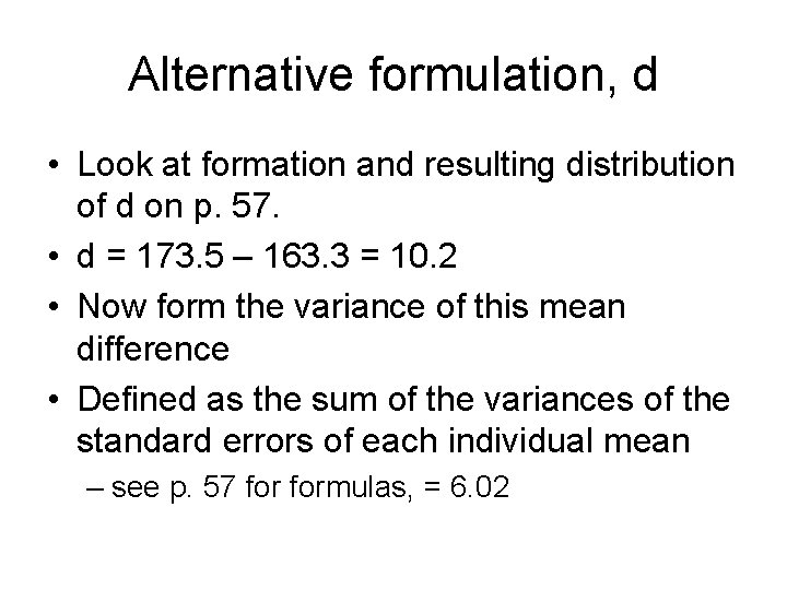
Alternative formulation, d • Look at formation and resulting distribution of d on p. 57. • d = 173. 5 – 163. 3 = 10. 2 • Now form the variance of this mean difference • Defined as the sum of the variances of the standard errors of each individual mean – see p. 57 formulas, = 6. 02

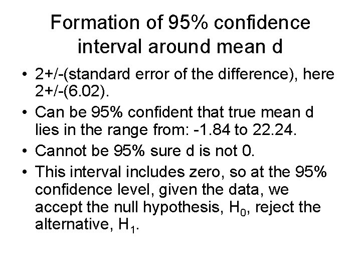
Formation of 95% confidence interval around mean d • 2+/-(standard error of the difference), here 2+/-(6. 02). • Can be 95% confident that true mean d lies in the range from: -1. 84 to 22. 24. • Cannot be 95% sure d is not 0. • This interval includes zero, so at the 95% confidence level, given the data, we accept the null hypothesis, H 0, reject the alternative, H 1.

Cholesterol Example, contd. • Look at raw data by frequency (p. 57) • Understand that the two, equivalent, ways of framing the hypothesis concern either: • 1. The degree of overlap between the confidence interval we construct around the mean of men’s cholesterol observations, and that we construct around the mean of woman’s cholesterol observations, and seeing by how much they overlap, or, • 2. Whether the distribution of d contains 0 in the confidence interval we construct around its mean

Construction of the true confidence level • We know we can meet the requirement of 1+/(stnd. error of the mean) • Would give us a 66% level of confidence because 66% of the area under the standard normal curve lie in this range • Here = 10. 2+/- 6. 02: from 4. 18 to 16. 22 • But we cannot meet the criteria for a 95% level of confidence – somewhere between 95% and 66% • So there is weak support for the contention that cholesterol varies by gender

Or could consult a t-statistic • t = mean/(it’s standard error) • “critical values of t, depend on the size of the sample, and gives a significance value at which a particular sample mean can be assumed to be different than zero • here t = 10. 2/6. 02 = 1. 69 • for a sample of 30, a t–statistic of 1. 69, is significant at approximately the 90% level

Automate the calculation • Use Excel • Convenient for “big” data sets, with many observations • Use it to calculate: – 1. avg. cholesterol, – 2. differences from avg. , – 3. differences squared – 4. squared differences summed

Excel Computations, contd. • Use a calculator and formula sheet for the rest • Calculate the variance and the standard deviations of the two samples • Calculate the stnd. error of each mean • Then calculate the stnd. error of the difference in means