Variables Graphs and Distribution Shapes Data Analysis Statistics

Variables, Graphs and Distribution Shapes

Data Analysis Statistics is the science of data. Data Analysis is the process of organizing, displaying, summarizing, and asking questions about data. Individuals ü objects described by a set of data • People, Animals, or Things Variable ü any characteristic of an individual Categorical Variable ü places an individual into one of several groups or categories. Not every variable that takes number values is quantitative! Ex: zip code Why would we want to find an average zip code? Quantitative Variable ü takes numerical values for which it makes sense to find an average.

Categorical Variables Frequency Table Format Variable Count of Stations Format Percent of Stations Adult Contemporary 1556 Adult Contemporary Adult Standards 1196 Adult Standards 8. 6 Contemporary Hit 4. 1 Contemporary Hit 569 11. 2 Country 2066 Country 14. 9 News/Talk 2179 News/Talk 15. 7 Oldies 1060 Oldies Religious 2014 Religious Rock 869 Spanish Language 750 Other Formats Values Relative Frequency Table Total 1579 13838 14. 6 Count Spanish Language Total ü Relative Frequency means % 7. 7 Rock Other Formats ü Frequency means count Percent 6. 3 5. 4 11. 4 99. 9 Due to roundoff error

Displaying Categorical Data Frequency tables can be difficult to read. Sometimes it is easier to analyze a distribution by displaying it with a bar graph or pie chart. Percent of Stations Total 14. 9 News/Talk 15. 7 13838 Other Total 99. 9 r he Ot sh Sp a 11. 4 ni ck Ro io Re lig di Ol Ta s/ Ne w Other Formats us 5. 4 es Spanish Language lk 6. 3 try Rock ar ra Spanish 1579 14. 6 un 0 Religious it Rock 750 7. 7 Co 500 ry 2014 Religious 869 t S ta nd 8%Spanish Language 16% Other Formats Country Oldies po Rock 15% 4. 1 ul Religious 1060 Oldies Ad 15% 1000 te m Oldies News/Talk 2179 on News/Talk 4% Contemporary Hit ry h Country 1500 8. 6 ra Country 2066 11. 2 Adult Standards ds 9% t C 6% Contemporary Hit 1196 Contemporary hit 569 Percent of Stations Adult Contemporary 2000 ul 5% 1556 Adult Standards Format em po Adult Contemporary 11% Adult Standards 2500 nt Adult Contemporary Count of Stations Ad Format Count of Stations Relative Frequency Table Co Frequency Table

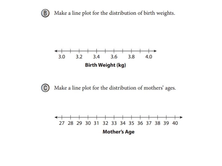
Displaying Quantitative Data Useful graphs include: a line plot, a histogram, a stem and leaf plot, and a box-and-whisker plot.

Distributions “Raw” data values are simply presented in an unorganized list. Organizing the data values by using the frequency with which they occur results in a distribution of the data. A distribution may be presented as a frequency table or as a data display. Data displays reveal the shape of a distribution.

The table gives data about a random sample of 20 babies born at a hospital.

Seeing the Shape of a Distribution • As you just saw, data distributions can have various shapes. Some of these shapes are given names in statistics. • A distribution whose shape is basically level (that is, it looks like a rectangle) is called a uniform distribution • A distribution that is mounded in the middle with symmetric “tails” at each end (that is, it looks bell-shaped) is called a normal distribution • A distribution that is mounded but not symmetric because one “tail” is much longer than the other is called a skewed distribution. When the longer “tail” is on the left, the distribution is said to be skewed left. When the longer “tail” is on the right, the distribution is said to be skewed right.

Real World Video • Module 23

Stem and Leaf Plot • A Stem and Leaf Plot is a special table where each data value is split into a "stem" (the first digit or digits) and a "leaf" (usually the last digit). The "stem" values are listed down, and the • Ex: "leaf" values go right (or left) from the stem values. The "stem" is used to group the scores and each "leaf" shows the individual scores within each group. It is OK to repeat a leaf value. Leaves are typically arranged in increasing order. If we turn the plot on its side, we can see the distribution of data.

Stem and Leaf Discussion • . . Probability and Statistics6 th Day- GraphsStem and Leaf Discussion. pdf

Box-and-Whisker Plot • Statistics assumes that your data points (the numbers in your list) are clustered around some central value. The "box" in the box-and-whisker plot contains, and thereby highlights, the middle half of these data points. • Steps: 1. Order your data in numerical order 2. Find the median of your data (divides the data into two halves) • If you have an even number of data, average the 2 middle values 3. Find the median of those two halves (the Upper Quartile and Lower Quartile) • Don’t re-use the median value 4. Find the maximum and minimum value 5. Draw the box-and-whisker plot Note: The median, upper quartile and lower quartiles divide the entire data set into quarters, called "quartiles". Q 1 - lower quartile Q 2 - median Q 3 - upper quartile

Ex: Draw a box-and-whisker plot for the following data set: 4. 3, 5. 1, 3. 9, 4. 5, 4. 4, 4. 9, 5. 0, 4. 7, 4. 1, 4. 6, 4. 4, 4. 3, 4. 8, 4. 4, 4. 2, 4. 5, 4. 4 • Continued…

Ex (Cont. ): Now I'll mark off the minimum and maximum values, and Q 1, Q 2, and Q 3: The "box" part of the plot goes from Q 1 to Q 3: And then the "whiskers" are drawn to the endpoints:

Ex: Draw the box-and-whisker plot for the following data set: 77, 79, 80, 86, 87, 94, 99 •

Notes: •

Box-and-Whisker Discussion • . . Probability and Statistics6 th Day- GraphsBoxand-Whisker Discussion. pdf