Variable elimination The basic ideas Move summations inwards

Variable elimination: The basic ideas § Move summations inwards as far as possible § P(B | j, m) = α e, a P(B) P(e) P(a|B, e) P(j|a) P(m|a) § = α P(B) e P(e) a P(a|B, e) P(j|a) P(m|a) § Do the calculation from the inside out § I. e. , sum over a first, then sum over e § Problem: P(a|B, e) isn’t a single number, it’s a bunch of different numbers depending on the values of B and e § Solution: use arrays of numbers (of various dimensions) with appropriate operations on them; these are called factors 1
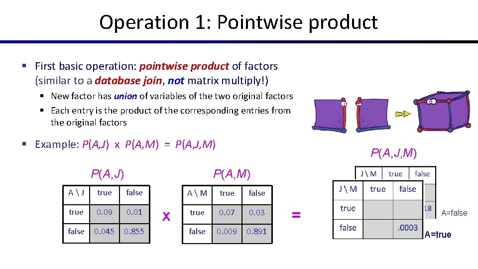
Operation 1: Pointwise product § First basic operation: pointwise product of factors (similar to a database join, not matrix multiply!) § New factor has union of variables of the two original factors § Each entry is the product of the corresponding entries from the original factors § Example: P(A, J) x P(A, M) = P(A, J, M) P(A, M) AJ true false true 0. 09 0. 01 false 0. 045 0. 855 x AM true false true 0. 07 0. 03 false 0. 009 0. 891 = A=false A=true
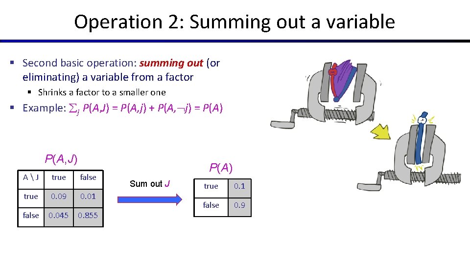
Operation 2: Summing out a variable § Second basic operation: summing out (or eliminating) a variable from a factor § Shrinks a factor to a smaller one § Example: j P(A, J) = P(A, j) + P(A, j) = P(A) P(A, J) AJ true false true 0. 09 0. 01 false 0. 045 0. 855 P(A) Sum out J true 0. 1 false 0. 9
Variable Elimination

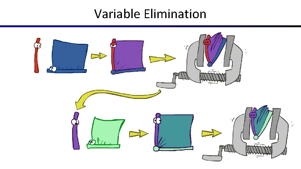
Variable Elimination § Query: P(Q|e) § Start with initial factors: § Local CPTs (but instantiated by evidence) § For each hidden variable Hj § Sum out Hj from the product of all factors mentioning Hj § Join all remaining factors and normalize Xα
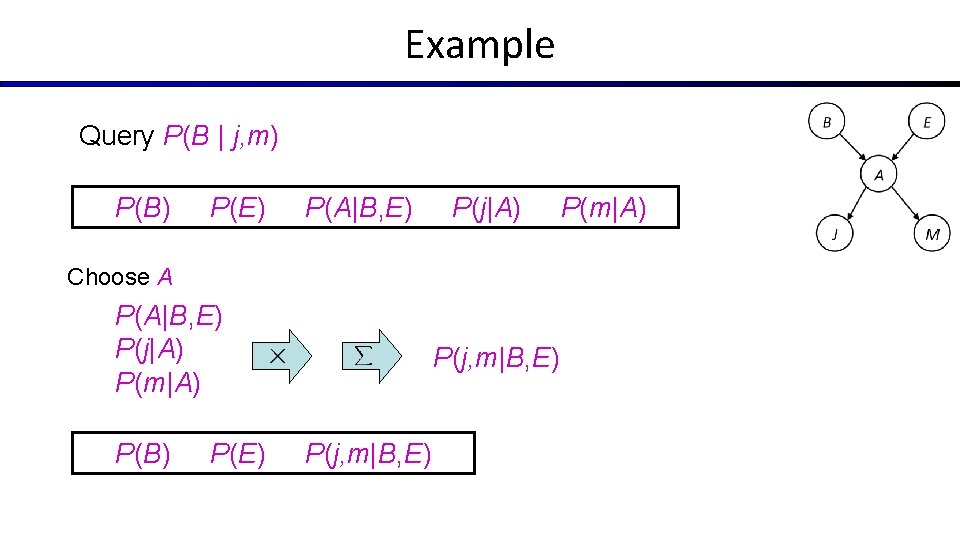
Example Query P(B | j, m) P(B) P(E) P(A|B, E) P(j|A) Choose A P(A|B, E) P(j|A) P(m|A) P(B) P(E) P(j, m|B, E) P(m|A)

Example P(B) P(E) P(j, m|B, E) Choose E P(E) P(j, m|B, E) P(B) P(j, m|B) Finish with B P(B) P(j, m|B) P(j, m, B) Normalize P(B | j, m)
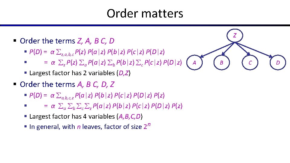
Order matters Z § Order the terms Z, A, B C, D § P(D) = α z, a, b, c P(z) P(a|z) P(b|z) P(c|z) P(D|z) § = α z P(z) a P(a|z) b P(b|z) c P(c|z) P(D|z) § Largest factor has 2 variables (D, Z) § Order the terms A, B C, D, Z § P(D) = α a, b, c, z P(a|z) P(b|z) P(c|z) P(D|z) P(z) § = α a b c z P(a|z) P(b|z) P(c|z) P(D|z) P(z) § Largest factor has 4 variables (A, B, C, D) § In general, with n leaves, factor of size 2 n A B C D
VE: Computational and Space Complexity § The computational and space complexity of variable elimination is determined by the largest factor (and it’s space that kills you) § The elimination ordering can greatly affect the size of the largest factor. § E. g. , previous slide’s example 2 n vs. 2 § Does there always exist an ordering that only results in small factors? § No!

Worst Case Complexity? Reduction from SAT 0. 5 W X Y Z C 1 C 2 S C 3 § Variables: W, X, Y, Z § CNF clauses: § § § C 1 = W v X v Y C 2 = Y v Z v W C 3 = X v Y v Z § Sentence S = C 1 C 2 C 3 § P(S) > 0 iff S is satisfiable § => NP-hard § P(S) = K x 0. 5 n where K is the number of satisfying assignments for clauses § => #P-hard
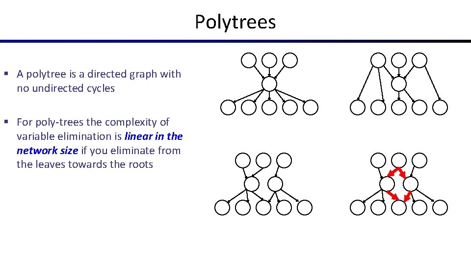
Polytrees § A polytree is a directed graph with no undirected cycles § For poly-trees the complexity of variable elimination is linear in the network size if you eliminate from the leaves towards the roots

CS 188: Artificial Intelligence Bayes Nets: Approximate Inference Instructors: Stuart Russell and Dawn Song University of California, Berkeley
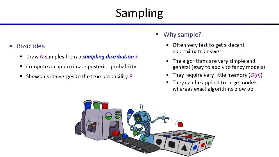
Sampling § Why sample? § Basic idea § Draw N samples from a sampling distribution S § Compute an approximate posterior probability § Show this converges to the true probability P § Often very fast to get a decent approximate answer § The algorithms are very simple and general (easy to apply to fancy models) § They require very little memory (O(n)) § They can be applied to large models, whereas exact algorithms blow up
Example § Suppose you have two agent programs A and B for Monopoly § What is the probability that A wins? § Method 1: § Let s be a sequence of dice rolls and Chance and Community Chest cards § Given s, the outcome V(s) is determined (1 for a win, 0 for a loss) § Probability that A wins is s P(s) V(s) § Problem: infinitely many sequences s ! § Method 2: § Sample N sequences from P(s) , play N games (maybe 100) § Probability that A wins is roughly 1/N i V(si) i. e. , fraction of wins in the sample 15
Sampling basics: discrete (categorical) distribution § To simulate a biased d-sided coin: § Step 1: Get sample u from uniform distribution over [0, 1) § E. g. random() in python § Step 2: Convert this sample u into an outcome for the given distribution by associating each outcome x with a P(x) -sized sub-interval of [0, 1) § Example C red green blue P(C) 0. 6 0. 1 0. 3 0. 0 u < 0. 6, C=red 0. 6 u < 0. 7, C=green 0. 7 u < 1. 0, C=blue § If random() returns u = 0. 83, then the sample is C = blue § E. g, after sampling 8 times: 0. 6 0. 1 0. 3
Sampling in Bayes Nets § Prior Sampling § Rejection Sampling § Likelihood Weighting § Gibbs Sampling
Prior Sampling
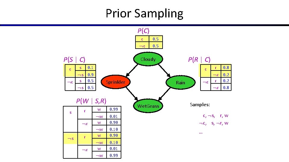
Prior Sampling P(C) c c P(S | C) s r r 0. 8 r 0. 2 c r 0. 2 r 0. 8 c Sprinkler P(W | S, R) s P(R | C) Cloudy 0. 1 s 0. 9 c s 0. 5 c 0. 5 w w w w 0. 99 0. 01 0. 90 0. 10 0. 01 0. 99 Rain Wet. Grass r Samples: c, s, r, w c, s, r, w …
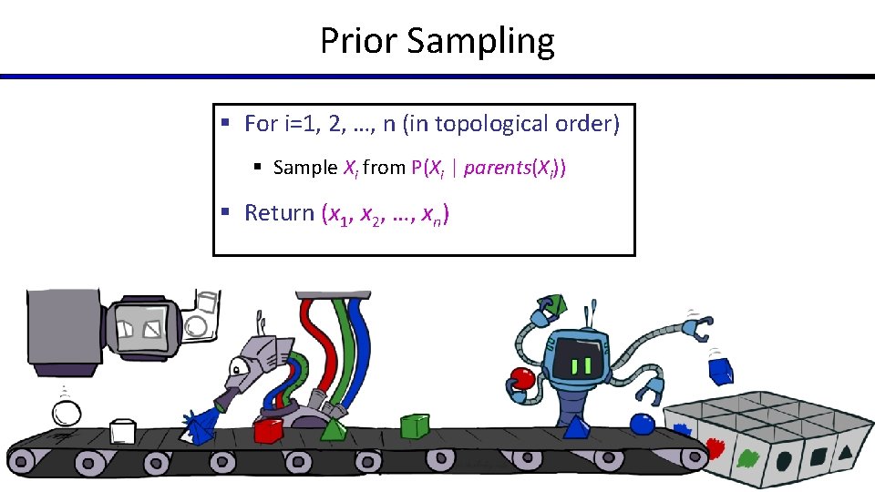
Prior Sampling § For i=1, 2, …, n (in topological order) § Sample Xi from P(Xi | parents(Xi)) § Return (x 1, x 2, …, xn)
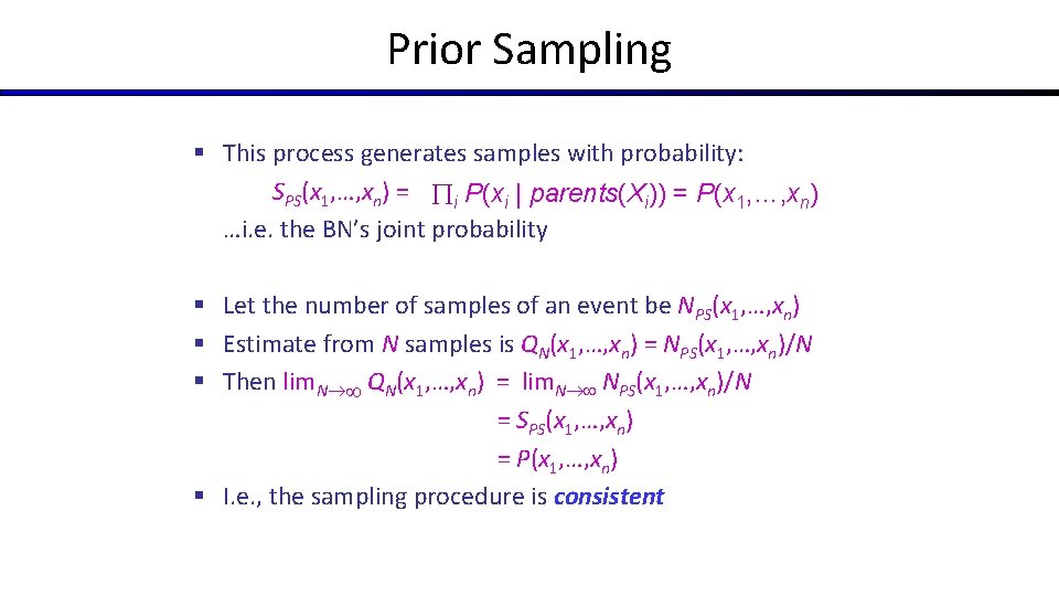
Prior Sampling § This process generates samples with probability: SPS(x 1, …, xn) = i P(xi | parents(Xi)) = P(x 1, …, xn) …i. e. the BN’s joint probability § Let the number of samples of an event be NPS(x 1, …, xn) § Estimate from N samples is QN(x 1, …, xn) = NPS(x 1, …, xn)/N § Then lim. N QN(x 1, …, xn) = lim. N NPS(x 1, …, xn)/N = SPS(x 1, …, xn) = P(x 1, …, xn) § I. e. , the sampling procedure is consistent
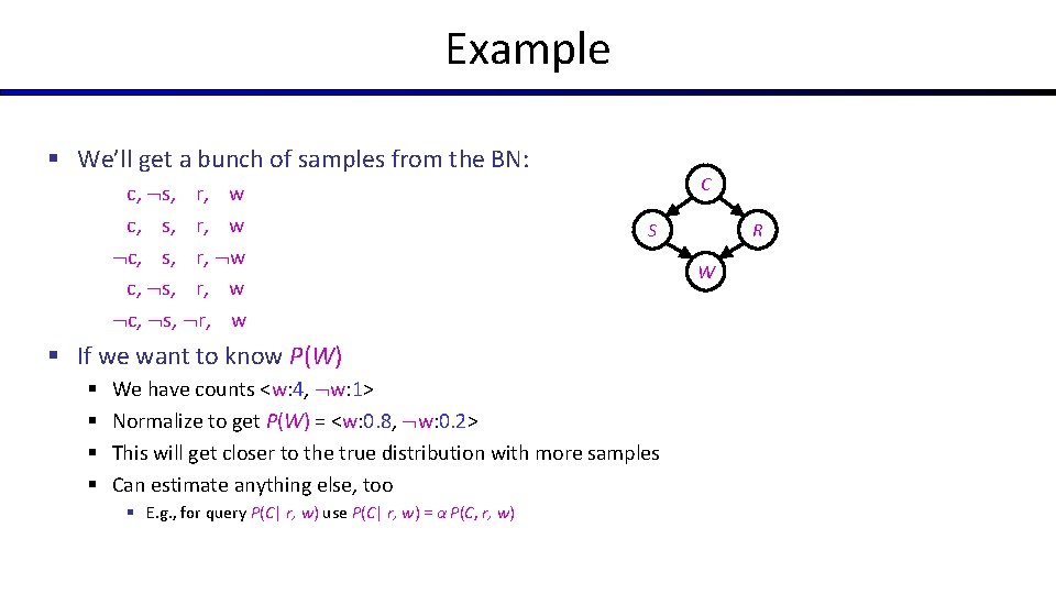
Example § We’ll get a bunch of samples from the BN: c, s, r, w c, s, r, w c, s, r, w c, s, r, w C S § If we want to know P(W) § § We have counts <w: 4, w: 1> Normalize to get P(W) = <w: 0. 8, w: 0. 2> This will get closer to the true distribution with more samples Can estimate anything else, too § E. g. , for query P(C| r, w) use P(C| r, w) = α P(C, r, w) R W
Rejection Sampling
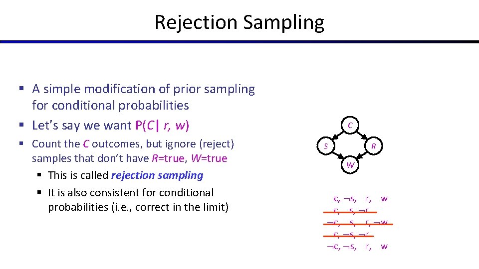
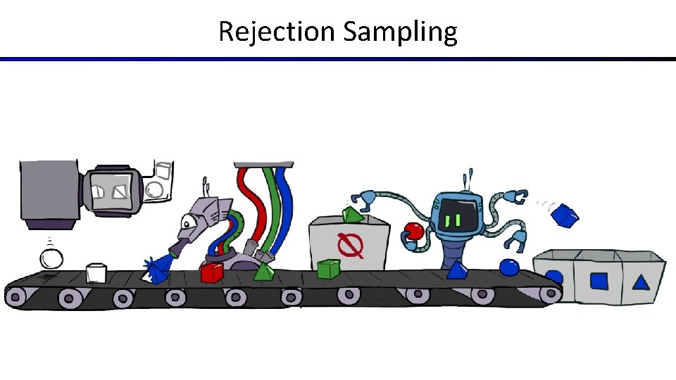
Rejection Sampling § A simple modification of prior sampling for conditional probabilities § Let’s say we want P(C| r, w) § Count the C outcomes, but ignore (reject) samples that don’t have R=true, W=true § This is called rejection sampling § It is also consistent for conditional probabilities (i. e. , correct in the limit) C S R W c, s, r, w c, s, r c, s, r, w c, s, r c, s, r, w
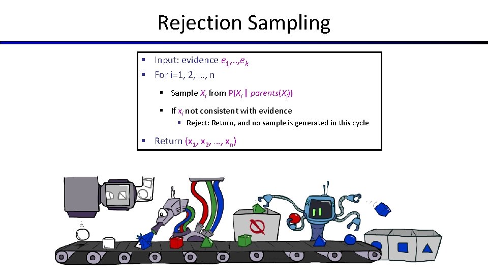
Rejection Sampling § Input: evidence e 1, . . , ek § For i=1, 2, …, n § Sample Xi from P(Xi | parents(Xi)) § If xi not consistent with evidence § Reject: Return, and no sample is generated in this cycle § Return (x 1, x 2, …, xn)
Likelihood Weighting
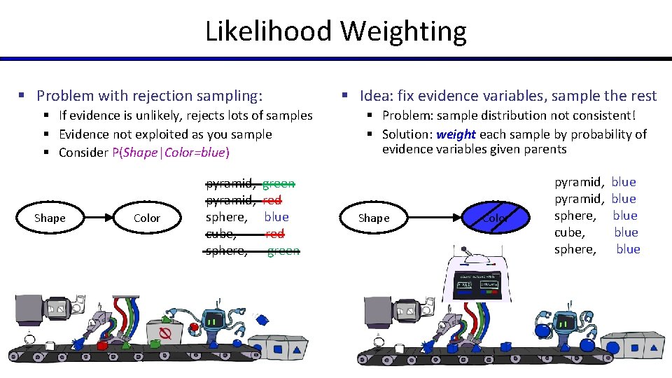
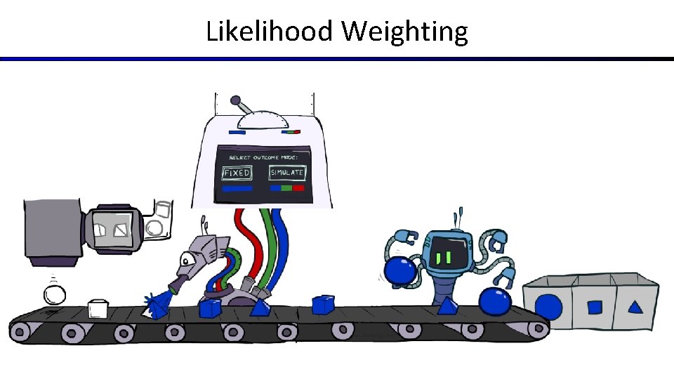
Likelihood Weighting § Problem with rejection sampling: § If evidence is unlikely, rejects lots of samples § Evidence not exploited as you sample § Consider P(Shape|Color=blue) Shape Color pyramid, sphere, cube, sphere, green red blue red green § Idea: fix evidence variables, sample the rest § Problem: sample distribution not consistent! § Solution: weight each sample by probability of evidence variables given parents Shape Color pyramid, sphere, cube, sphere, blue blue
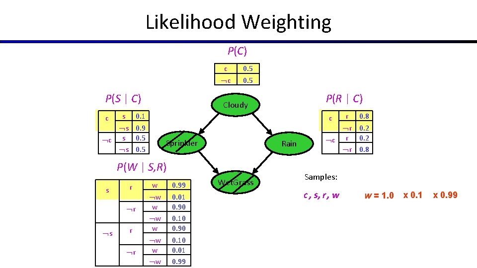
Likelihood Weighting P(C) c c P(S | C) s r r 0. 8 r 0. 2 c r 0. 2 r 0. 8 c Sprinkler Rain P(W | S, R) s P(R | C) Cloudy 0. 1 s 0. 9 c s 0. 5 c 0. 5 w w w w 0. 99 0. 01 0. 90 0. 10 0. 01 0. 99 Wet. Grass r Samples: c , s, r , w w = 1. 0 x 0. 1 x 0. 99
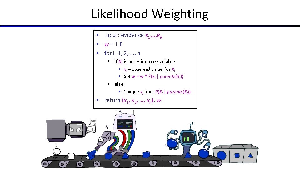
Likelihood Weighting § Input: evidence e 1, . . , ek § w = 1. 0 § for i=1, 2, …, n § if Xi is an evidence variable § xi = observed valuei for Xi § Set w = w * P(xi | parents(Xi)) § else § Sample xi from P(Xi | parents(Xi)) § return (x 1, x 2, …, xn), w
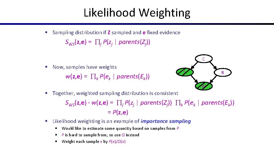
Likelihood Weighting § Sampling distribution if Z sampled and e fixed evidence SWS(z, e) = j P(zj | parents(Zj)) Cloudy C § Now, samples have weights w(z, e) = k P(ek | parents(Ek)) S R W § Together, weighted sampling distribution is consistent SWS(z, e) w(z, e) = j P(zj | parents(Zj)) k P(ek | parents(Ek)) = P(z, e) § Likelihood weighting is an example of importance sampling § Would like to estimate some quantity based on samples from P § P is hard to sample from, so use Q instead § Weight each sample x by P(x)/Q(x)
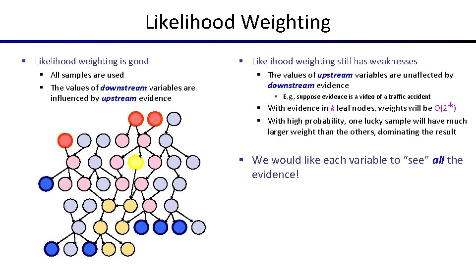
Likelihood Weighting § Likelihood weighting is good § All samples are used § The values of downstream variables are influenced by upstream evidence § Likelihood weighting still has weaknesses § The values of upstream variables are unaffected by downstream evidence § E. g. , suppose evidence is a video of a traffic accident § With evidence in k leaf nodes, weights will be O(2 -k) § With high probability, one lucky sample will have much larger weight than the others, dominating the result § We would like each variable to “see” all the evidence!
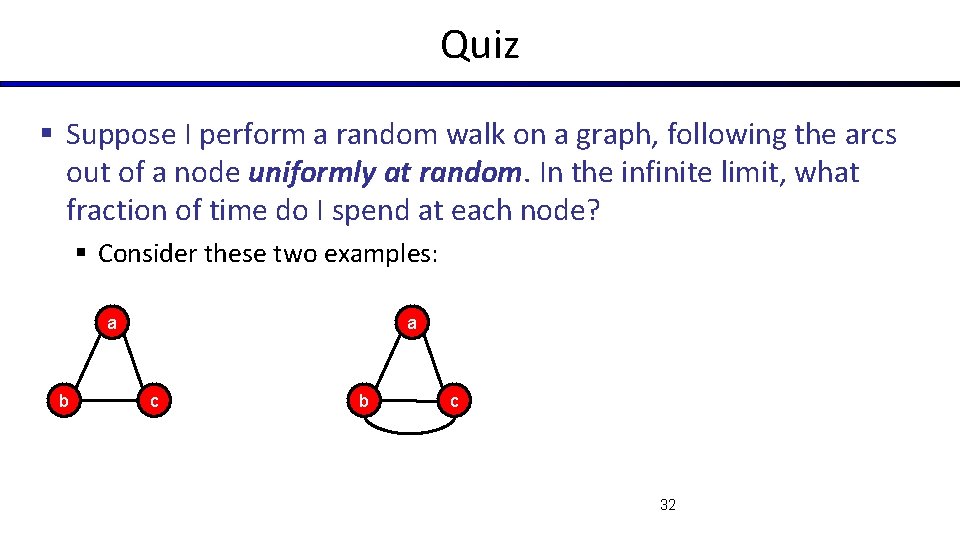
Quiz § Suppose I perform a random walk on a graph, following the arcs out of a node uniformly at random. In the infinite limit, what fraction of time do I spend at each node? § Consider these two examples: a b a c b c 32
- Slides: 31