Valuing Bonds with Embedded Options 1 Traditional Valuation

Valuing Bonds with Embedded Options 1

Traditional Valuation Methodology for Callable Bonds • When a bond is callable, the practice has been to calculate a yield to worst, which is the smallest of the yield to maturity and the yield to call for all possible call dates. • The yield to call (like the yield to maturity) assumes that all cash flows can be reinvested at the computed yield—in this case the yield to call—until the assumed call date. • Moreover, the yield to call assumes that i. the investor will hold the bond to the assumed call date ii. the issuer will call the bond on that date. • Often, these underlying assumptions about the yield to call are unrealistic because they do not take into account how an investor will reinvest the proceeds if the issue is called. 2

Price-Yield Relationship for a Callable Bond • As yields in the market decline, the likelihood that yields will decline further so that the issuer will benefit from calling the bond increases. • The exact yield level at which investors begin to view the issue likely to be called may not be known, but we do know that there is some level, say y*. • At yield levels below y*, the price-yield relationship for the callable bond departs from the price-yield relationship for the noncallable bond. 3

Callable Bonds and Their Investment Characteristics • The presence of a call option results in two disadvantages to the bondholder: i. callable bonds expose bondholders to reinvestment risk ii. price appreciation potential for a callable bond in a declining interest-rate environment is limited (This phenomenon for a callable bond is referred to as price compression. ) • If the investor receives sufficient potential compensation in the form of a higher potential yield, an investor would be willing to accept call risk. 4

Price-Yield Relationship for a Callable Bond • Negative convexity means that the price appreciation will be less than the price depreciation for a large change in yield of a given number of basis points. • For a bond that is option-free and displays positive convexity, the price appreciation will be greater than the price depreciation for a large change in yield. • It is important to understand that a bond can still trade above its call price even if it is highly likely to be called. 5

Price-Yield Relationship for a Callable Bond • The price–yield relationship for an option-free bond is convex. • The convex curve a–a' is the price–yield relationship for the noncallable (option-free) bond. • The unusual shaped curve denoted by a–b is the price–yield relationship for the callable bond. • The reason for the shape of the price–yield relationship for the callable bond is as follows. • When the prevailing market yield for comparable bonds is higher than the coupon interest, it is unlikely that the issuer will call the bond. 6

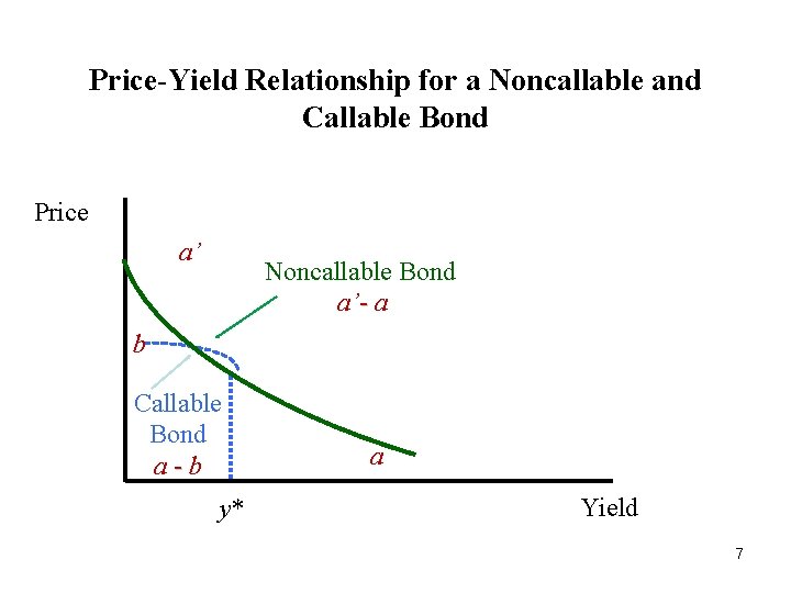
Price-Yield Relationship for a Noncallable and Callable Bond Price a’ Noncallable Bond a’- a b Callable Bond a-b y* a Yield 7

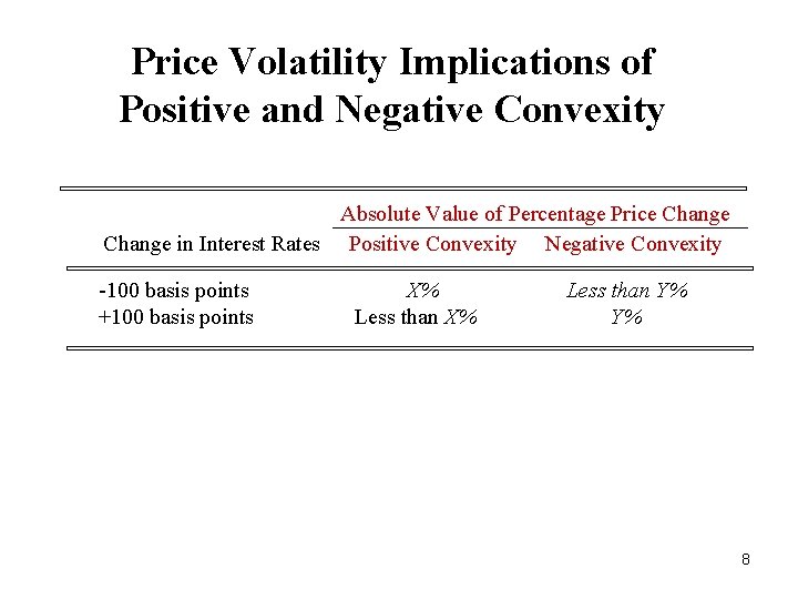
Price Volatility Implications of Positive and Negative Convexity Absolute Value of Percentage Price Change in Interest Rates Positive Convexity Negative Convexity -100 basis points +100 basis points X% Less than Y% Y% 8

Components of a Bond with an Embedded Option • A callable bond is a bond in which the bondholder has sold the issuer a call option that allows the issuer to repurchase the contractual cash flows of the bond from the time the bond is first callable until the maturity date. • The owner of a callable bond is entering into two separate transactions: i. buys a noncallable bond from the issuer for which she pays some price ii. sells the issuer a call option for which she receives the option price • A callable bond is equal to the price of the two components parts; that is, callable bond price = noncallable bond price – call option price 9

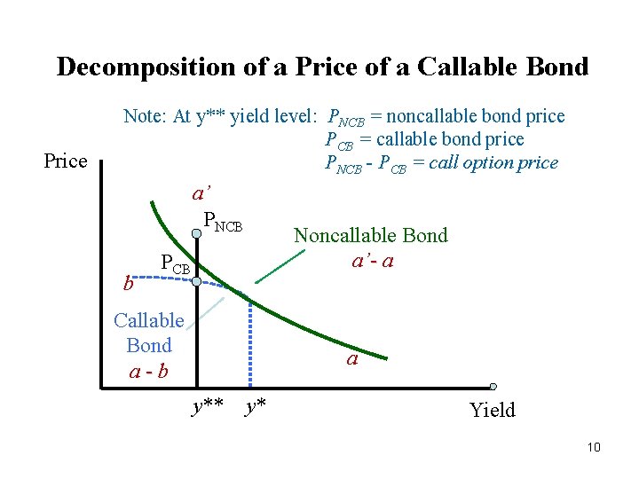
Decomposition of a Price of a Callable Bond Price Note: At y** yield level: PNCB = noncallable bond price PCB = callable bond price PNCB - PCB = call option price a’ PNCB b Noncallable Bond a’- a PCB Callable Bond a-b a y** y* Yield 10

Components of a Bond with an Embedded Option • The logic applied to callable bonds can be similarly applied to putable bonds. • A putable bond can be broken into two separate transactions. i. The investor buys a noncallable bond. ii. The investor buys an option from the issuer that allows the investor to sell the bond to the issuer. • The price of a putable bond is then putable bond price = non-putable bond price + put option price 11

Valuation Model • Depending on the structure of the security to be analyzed, three models can be used to account for the valuation effect of embedded options. i. The first model is for a bond that is not a mortgage-backed security or asset-backed security and which can be exercised at more than one time over its life. ii. The second case is a bond with an embedded option where the option can be exercised only once. iii. The third model is for a mortgage-backed security or certain types of asset-backed securities. 12

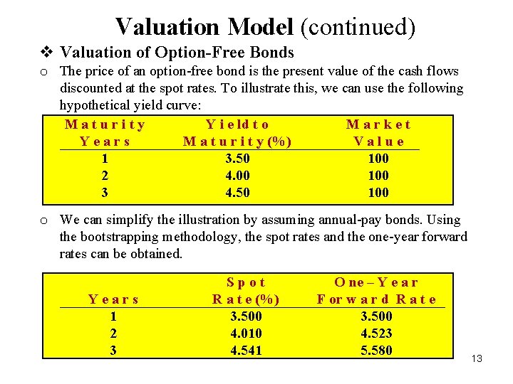
Valuation Model (continued) v Valuation of Option-Free Bonds o The price of an option-free bond is the present value of the cash flows discounted at the spot rates. To illustrate this, we can use the following hypothetical yield curve: Maturity Y i e ld t o Market Years M a t u r i t y (%) Value 1 3. 50 100 2 4. 00 100 3 4. 50 100 o We can simplify the illustration by assuming annual-pay bonds. Using the bootstrapping methodology, the spot rates and the one-year forward rates can be obtained. Years 1 2 3 Spot R a t e (%) 3. 500 4. 010 4. 541 O ne – Y e a r F or w a r d R a t e 3. 500 4. 523 5. 580 13

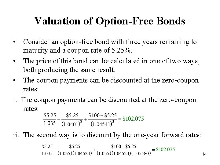
Valuation of Option-Free Bonds • Consider an option-free bond with three years remaining to maturity and a coupon rate of 5. 25%. • The price of this bond can be calculated in one of two ways, both producing the same result. • The coupon payments can be discounted at the zero-coupon rates: ii. The second way is to discount by the one-year forward rates: 14

Introducing Interest-Rate Volatility • When we allow for embedded options, consideration must be given to interest-rate volatility. • This can be done by introducing an interest-rate tree, also referred to as an interest-rate lattice. • This tree is nothing more than a graphical depiction of the one -period forward rates over time based on some assumed interest-rate model and interest-rate volatility. 15

Interest-Rate Model • An interest-rate model does this by making an assumption about the relationship between the level of short-term interest rates and interest-rate volatility (e. g. , standard deviation of interest rates). • The interest-rate models commonly used are arbitrage-free models based on how short-term interest rates can evolve (i. e. , change) over time. • The interest-rate models based solely on movements in the short-term interest rate are referred to as one-factor models. • More complex models would consider how more than one interest rate changes over time. 16

Interest-Rate Lattice • It is assumed that interest rates can realize one of two possible rates in the next period. • In the valuation model we present in this chapter, we will use the binomial model. • Valuation models that assume that interest rates can take on three possible rates in the next period are called trinomial models. 17

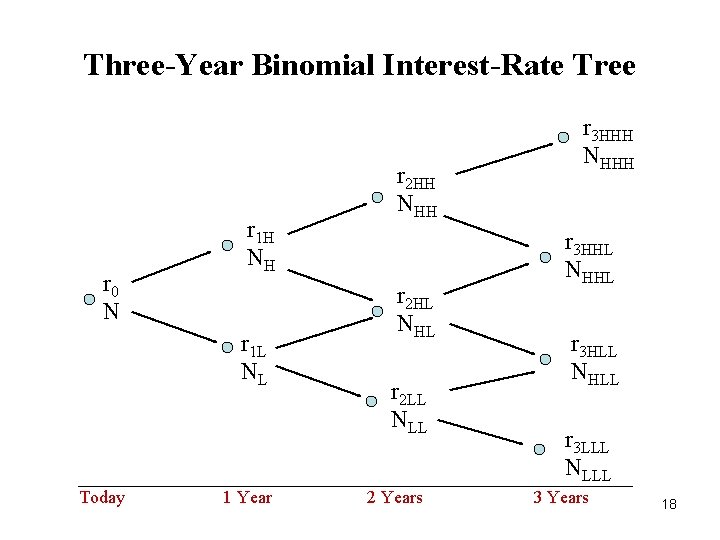
Three-Year Binomial Interest-Rate Tree r 0 N r 1 H NH r 1 L NL Today 1 Year r 2 HH NHH r 2 HL NHL r 2 LL NLL 2 Years r 3 HHH NHHH r 3 HHL NHHL r 3 HLL NHLL r 3 LLL NLLL 3 Years 18

Interest-Rate Lattice • Each node is labeled with an N, representing node, and a subscript that indicates the path that one-year forward rates took to get to that node. • H represents the higher of the two forward rates and L the lower of the two forward rates from the preceding year. • For example, node NHH means that to get to that node the following path for one-year rates occurred: The one-year rate realized is the higher of the two rates in the first year and then the higher of the one-year rates in the second year 19

Interest-Rate Lattice • Before we go on to show to use this binomial interest-rate tree to value bonds, we first need to focus on i. what the volatility parameter ( ) in the expression e 2 represents ii. how to find the value of the bond at each node 20

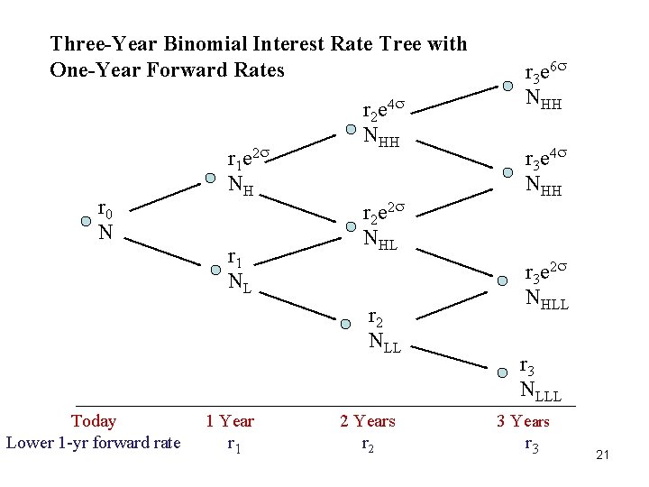
Three-Year Binomial Interest Rate Tree with One-Year Forward Rates r 0 N r 1 e 2 NH r 1 NL r 2 e 4 NHH r 2 e 2 NHL r 2 NLL Today Lower 1 -yr forward rate 1 Year r 1 2 Years r 2 r 3 e 6 NHH r 3 e 4 NHH r 3 e 2 NHLL r 3 NLLL 3 Years r 3 21

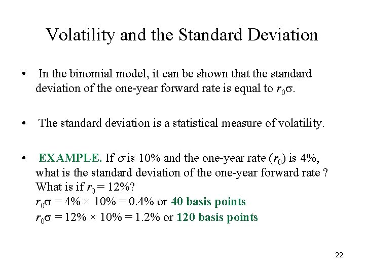
Volatility and the Standard Deviation • In the binomial model, it can be shown that the standard deviation of the one-year forward rate is equal to r 0. • The standard deviation is a statistical measure of volatility. • EXAMPLE. If is 10% and the one-year rate (r 0) is 4%, what is the standard deviation of the one-year forward rate ? What is if r 0 = 12%? r 0 = 4% × 10% = 0. 4% or 40 basis points r 0 = 12% × 10% = 1. 2% or 120 basis points 22

Determining the Value at a Node • Calculate the bond’s value at the two nodes to the right of the node where we want to obtain the bond’s value. • The cash flow at a node will be either i. the bond’s value if the short rate is the higher rate plus the coupon payment ii. the bond’s value if the short rate is the lower rate plus the coupon payment. • The value is the present value of the expected cash flows. 23

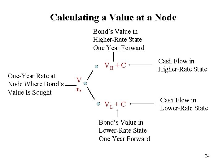
Calculating a Value at a Node Bond’s Value in Higher-Rate State One Year Forward One-Year Rate at Node Where Bond’s Value Is Sought VH + C Cash Flow in Higher-Rate State VL + C Cash Flow in Lower-Rate State V r* Bond’s Value in Lower-Rate State One Year Forward 24

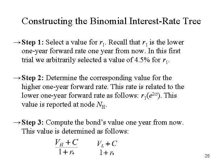
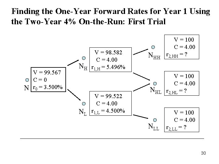
Constructing the Binomial Interest-Rate Tree → Step 1: Select a value for r 1. Recall that r 1 is the lower one-year forward rate one year from now. In this first trial we arbitrarily selected a value of 4. 5% for r 1. → Step 2: Determine the corresponding value for the higher one-year forward rate. This rate is related to the lower one-year forward rate as follows: r 1(e 2 ). This value is reported at node NH. → Step 3: Compute the bond’s value one year from now. This value is determined as follows: 25

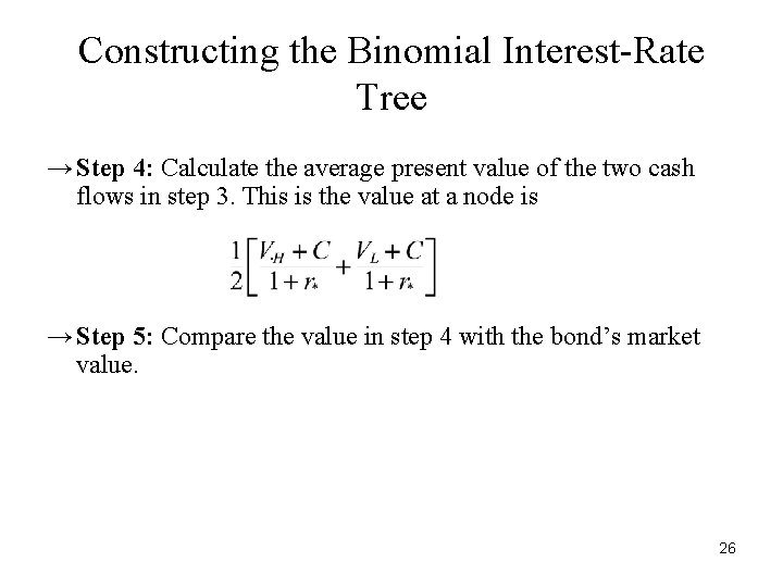
Constructing the Binomial Interest-Rate Tree → Step 4: Calculate the average present value of the two cash flows in step 3. This is the value at a node is. → Step 5: Compare the value in step 4 with the bond’s market value. 26

Constructing the Binomial Interest-Rate Tree → Step 5 (continued) : If the two values are the same, the r 1 used in this trial is the one we seek. If, instead, the value found in step 4 is not equal to the market value of the bond, this means that the value r 1 in this trial is not the one-period forward rate that is consistent with (1) the volatility assumption of 10%, (2) the process assumed to generate the one-year forward rate, and (3) the observed market value of the bond. In this case the five steps are repeated with a different value for r 1. 27

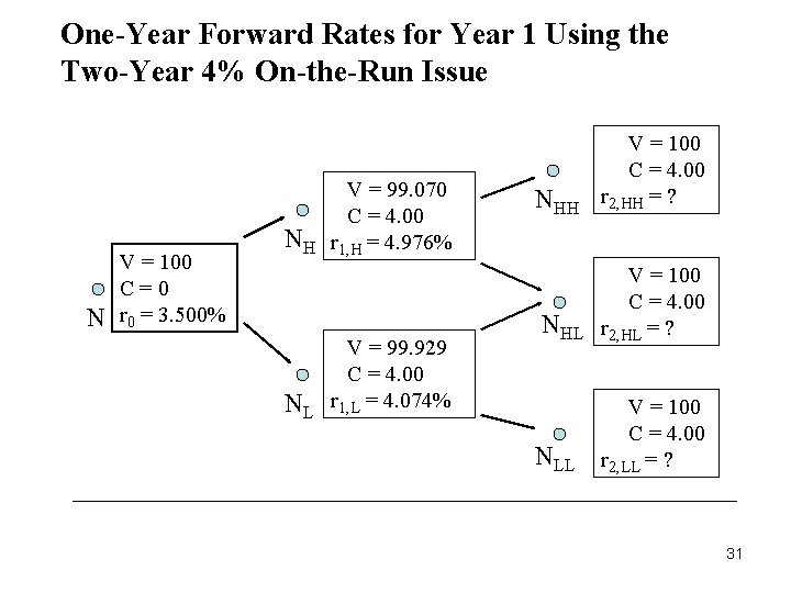
Constructing the Binomial Interest-Rate Tree → In this example, when r 1 is 4. 5% we get a value of $99. 567 in step 4, which is less than the observed market value of $100. Therefore, 4. 5% is too large and the five steps must be repeated, trying a lower value for r 1. → After we compute r 1, we want to determine r 2. The same five steps are used in an iterative process to find the one-year forward rate two years from now. But now our objective is as follows: Find the value for r 2 that will produce an average present value at node NH equal to the bond value at that node and will also produce an average present value at node NL equal to the bond value at that node. 28

Constructing the Binomial Interest-Rate Tree →When this value is found, we know that given the forward rate we found for r 1, the bond’s value at the root—the value of ultimate interest to us—will be the observed market price. →The binomial interest-rate tree constructed is said to be an arbitrage-free tree. It is so named because it fairly prices the on-the-run issues. 29

Finding the One-Year Forward Rates for Year 1 Using the Two-Year 4% On-the-Run: First Trial N V = 99. 567 C=0 r 0 = 3. 500% NH NL V = 98. 582 C = 4. 00 r 1, H = 5. 496% V = 99. 522 C = 4. 00 r 1, L = 4. 500% NHH V = 100 C = 4. 00 r 2, HH = ? NHL V = 100 C = 4. 00 r 2, HL = ? NLL V = 100 C = 4. 00 r 2, LL = ? 30

One-Year Forward Rates for Year 1 Using the Two-Year 4% On-the-Run Issue N V = 100 C=0 r 0 = 3. 500% NH NL V = 99. 070 C = 4. 00 r 1, H = 4. 976% V = 99. 929 C = 4. 00 r 1, L = 4. 074% NHH V = 100 C = 4. 00 r 2, HH = ? NHL V = 100 C = 4. 00 r 2, HL = ? NLL V = 100 C = 4. 00 r 2, LL = ? 31

Application to Valuing an Option-Free Bond • Consider a 5. 25% corporate bond that has two years remaining to maturity and is option-free. • Also assume that the issuer’s on-the-run yield curve is the one given earlier (as shown in the next page). • the various values in the discounting process and produces a bond value of $102. 075. 32

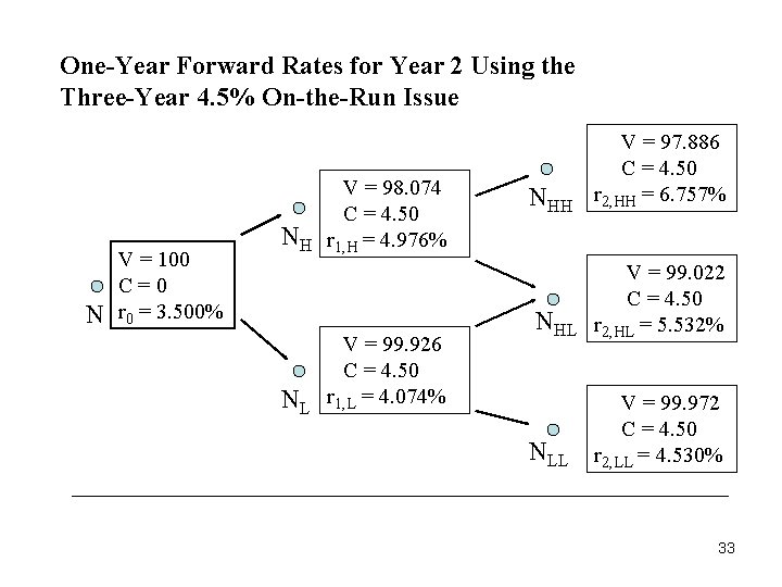
One-Year Forward Rates for Year 2 Using the Three-Year 4. 5% On-the-Run Issue N V = 100 C=0 r 0 = 3. 500% NH NL V = 98. 074 C = 4. 50 r 1, H = 4. 976% V = 99. 926 C = 4. 50 r 1, L = 4. 074% NHH V = 97. 886 C = 4. 50 r 2, HH = 6. 757% NHL V = 99. 022 C = 4. 50 r 2, HL = 5. 532% NLL V = 99. 972 C = 4. 50 r 2, LL = 4. 530% 33

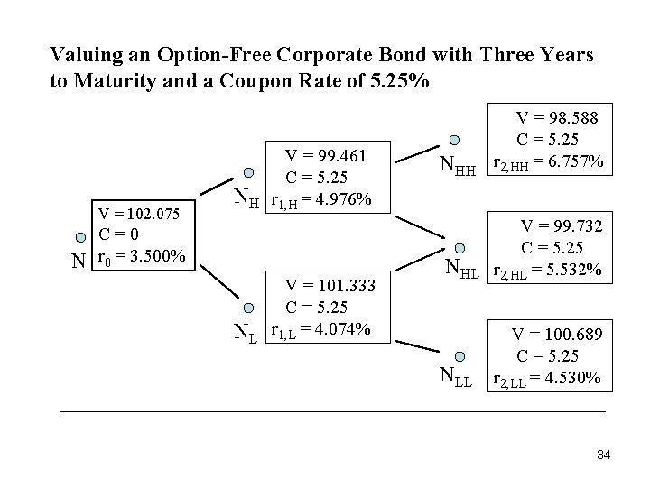
Valuing an Option-Free Corporate Bond with Three Years to Maturity and a Coupon Rate of 5. 25% V = 102. 075 N NH V = 99. 461 C = 5. 25 r 1, H = 4. 976% C=0 r 0 = 3. 500% NL V = 101. 333 C = 5. 25 r 1, L = 4. 074% NHH V = 98. 588 C = 5. 25 r 2, HH = 6. 757% NHL V = 99. 732 C = 5. 25 r 2, HL = 5. 532% NLL V = 100. 689 C = 5. 25 r 2, LL = 4. 530% 34

Valuing a Callable Corporate Bond • The valuation process for a callable corporate bond proceeds in the same fashion as in the case of an option-free bond but with one exception: When the call option may be exercised by the issuer, the bond value at a node must be changed to reflect the lesser of its value if it is not called (i. e. , the value obtained by applying the recursive valuation formula described previously) and the call price. • For example, consider a 5. 25% corporate bond with three years remaining to maturity that is callable in one year at $100. 35

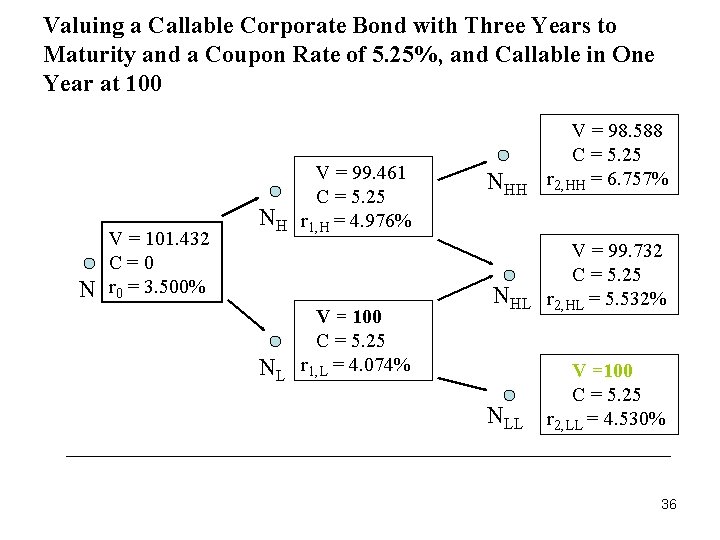
Valuing a Callable Corporate Bond with Three Years to Maturity and a Coupon Rate of 5. 25%, and Callable in One Year at 100 N V = 101. 432 C=0 r 0 = 3. 500% NH NL V = 99. 461 C = 5. 25 r 1, H = 4. 976% V = 100 C = 5. 25 r 1, L = 4. 074% NHH V = 98. 588 C = 5. 25 r 2, HH = 6. 757% NHL V = 99. 732 C = 5. 25 r 2, HL = 5. 532% NLL V =100 C = 5. 25 r 2, LL = 4. 530% 36

Determining the Call Option Value (or Option Cost) • The value of a callable bond is expressed as the difference between the value of a noncallable bond and the value of the call option. • This relationship can also be expressed as follows: value of a call option = value of a noncallable bond – value of a callable bond • In our previous illustration, the value of the noncallable bond is $102. 075 and the value of the callable bond is $101. 432, so the value of the call option is $0. 643. 37

Extension to Other Embedded Options • The bond valuation framework presented here can be used to analyze other embedded options, such as put options, caps and floors on floating-rate notes, and the optional accelerated redemption granted to an issuer in fulfilling its sinking fund requirement. 38

Valuing a Putable Corporate Bond • For example, consider a 5. 25% corporate bond with three years remaining to maturity that is putable in one year at $100. • Because the value of a non-putable bond can be expressed as the value of a putable bond minus the value of a put option on that bond, this means that value of a put option = value of a putable bond - value of a non-putable bond • The value of the option-free bond is $102. 075 and the value of the putable bond is $102. 523, so the value of the put option is $0. 488. 39

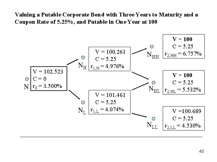
Valuing a Putable Corporate Bond with Three Years to Maturity and a Coupon Rate of 5. 25%, and Putable in One Year at 100 N V = 102. 523 C=0 r 0 = 3. 500% NH NL V = 100. 261 C = 5. 25 r 1, H = 4. 976% V = 101. 461 C = 5. 25 r 1, L = 4. 074% NHH V = 100 C = 5. 25 r 2, HH = 6. 757% NHL V = 100 C = 5. 25 r 2, HL = 5. 532% NLL V =100. 689 C = 5. 25 r 2, LL = 4. 530% 40

Incorporating Default Risk • The basic binomial model explained above can be extended to incorporate default risk. • The extension involves adjusting the expected cash flows for the probability of a payment default and the expected amount of cash that will be recovered when a default occurs. 41

Modeling Risk • The user of any valuation model is exposed to modeling risk. • This is the risk that the output of the model is incorrect because the assumptions upon which it is based are incorrect. 42

Effective Duration • There is a duration measure that is more appropriate for bonds with embedded options than the modified duration measure. • In general, the duration for any bond can be approximated as follows: Duration = P_ = price if yield is decreased by x basis points P+ = price if yield is increased by x basis points P 0 = initial price (per $100 of par value) ∆y (or dy) = change in rate used to calculate price (x basis points in decimal form) 43

Effective Duration • When the approximate duration formula is applied to a bond with an embedded option, the new prices at the higher and lower yield levels should reflect the value from the valuation model. • Duration calculated in this way is called effective duration or option-adjusted duration. 44

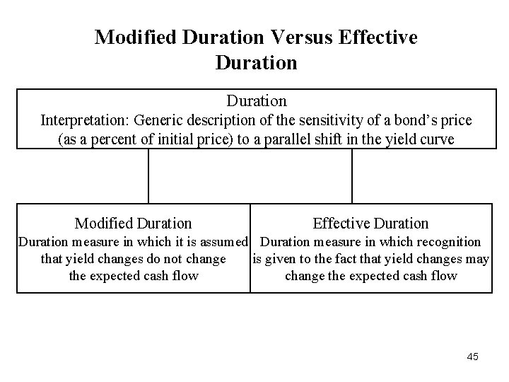
Modified Duration Versus Effective Duration Interpretation: Generic description of the sensitivity of a bond’s price (as a percent of initial price) to a parallel shift in the yield curve Modified Duration Effective Duration measure in which it is assumed Duration measure in which recognition that yield changes do not change is given to the fact that yield changes may the expected cash flow change the expected cash flow 45

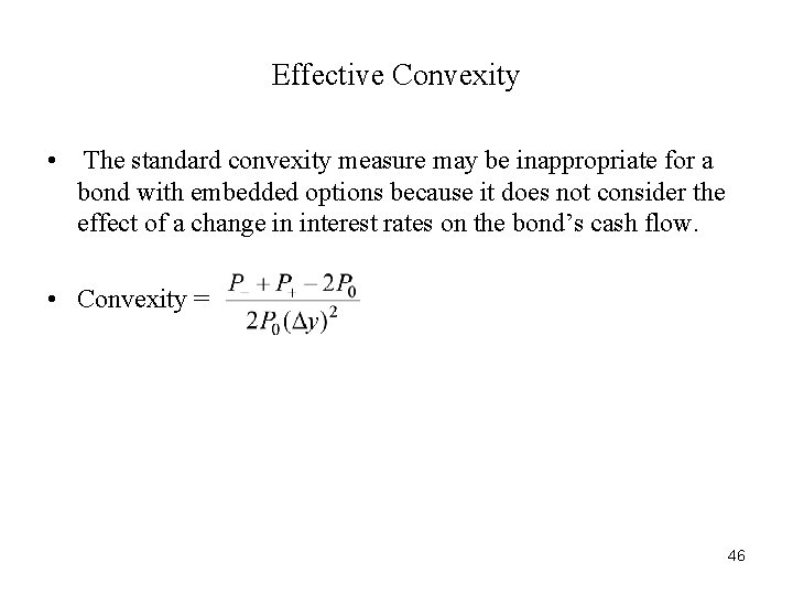
Effective Convexity • The standard convexity measure may be inappropriate for a bond with embedded options because it does not consider the effect of a change in interest rates on the bond’s cash flow. • Convexity = 46

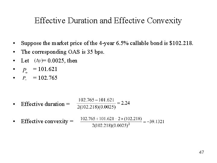
Effective Duration and Effective Convexity • Suppose the market price of the 4 -year 6. 5% callable bond is $102. 218. • The corresponding OAS is 35 bps. • Let = 0. 0025, then • = 101. 621 • = 102. 765 • Effective duration = • Effective convexity = 47