Value at Risk and Expected Shortfall Chapter 12

Value at Risk and Expected Shortfall Chapter 12 Risk Management and Financial Institutions 4 e, Chapter 12, Copyright © John C. Hull 2015 1

The Question Being Asked in Va. R “What loss level is such that we are X% confident it will not be exceeded in N business days? ” Risk Management and Financial Institutions 4 e, Chapter 12, Copyright © John C. Hull 2015 2

Va. R and Regulatory Capital l Regulators have traditionally used Va. R to calculate the capital they require banks to keep The market-risk capital has been based on a 10 -day Va. R estimated where the confidence level is 99% Credit risk and operational risk capital are based on a one-year 99. 9% Va. R Risk Management and Financial Institutions 4 e, Chapter 12, Copyright © John C. Hull 2015 3

Advantages of Va. R l l l It captures an important aspect of risk in a single number It is easy to understand It asks the simple question: “How bad can things get? ” Risk Management and Financial Institutions 4 e, Chapter 12, Copyright © John C. Hull 2015 4

Example 12. 1 (page 257) l l l The gain from a portfolio during six month is normally distributed with mean $2 million and standard deviation $10 million The 1% point of the distribution of gains is 2− 2. 33× 10 or − $21. 3 million The Va. R for the portfolio with a six month time horizon and a 99% confidence level is $21. 3 million. Risk Management and Financial Institutions 4 e, Chapter 12, Copyright © John C. Hull 2015 5

Example 12. 2 (page 258) l l All outcomes between a loss of $50 million and a gain of $50 million are equally likely for a one-year project The Va. R for a one-year time horizon and a 99% confidence level is $49 million Risk Management and Financial Institutions 4 e, Chapter 12, Copyright © John C. Hull 2015 6

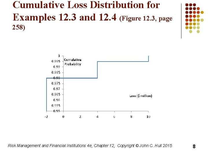
Examples 12. 3 and 12. 4 (page 258) l l A one-year project has a 98% chance of leading to a gain of $2 million, a 1. 5% chance of a loss of $4 million, and a 0. 5% chance of a loss of $10 million The Va. R with a 99% confidence level is $4 million What if the confidence level is 99. 9%? What if it is 99. 5%? Risk Management and Financial Institutions 4 e, Chapter 12, Copyright © John C. Hull 2015 7

Cumulative Loss Distribution for Examples 12. 3 and 12. 4 (Figure 12. 3, page 258) Risk Management and Financial Institutions 4 e, Chapter 12, Copyright © John C. Hull 2015 8

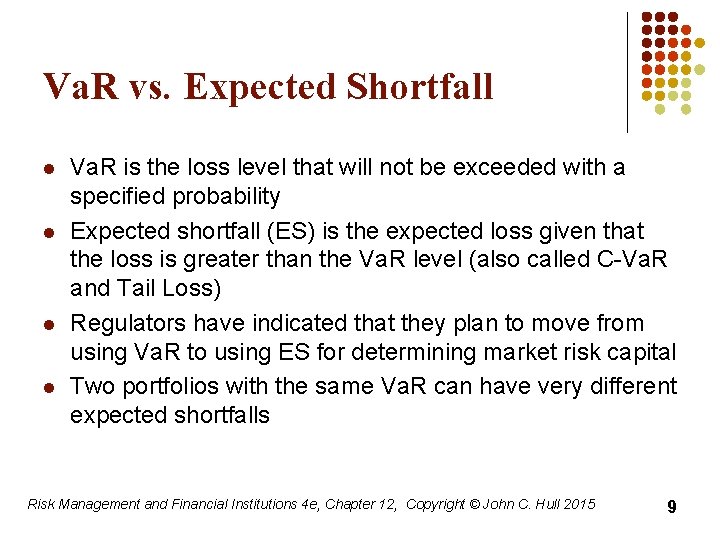
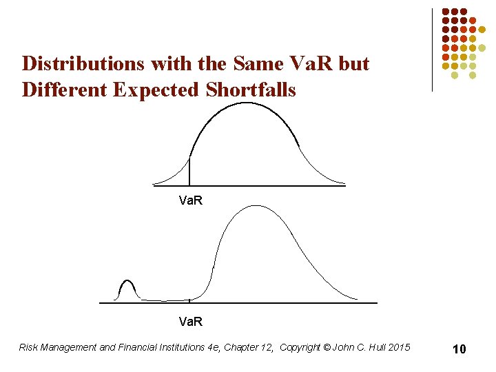
Va. R vs. Expected Shortfall l l Va. R is the loss level that will not be exceeded with a specified probability Expected shortfall (ES) is the expected loss given that the loss is greater than the Va. R level (also called C-Va. R and Tail Loss) Regulators have indicated that they plan to move from using Va. R to using ES for determining market risk capital Two portfolios with the same Va. R can have very different expected shortfalls Risk Management and Financial Institutions 4 e, Chapter 12, Copyright © John C. Hull 2015 9

Distributions with the Same Va. R but Different Expected Shortfalls Va. R Risk Management and Financial Institutions 4 e, Chapter 12, Copyright © John C. Hull 2015 10

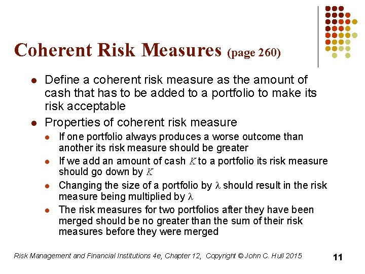
Coherent Risk Measures (page 260) l l Define a coherent risk measure as the amount of cash that has to be added to a portfolio to make its risk acceptable Properties of coherent risk measure l l If one portfolio always produces a worse outcome than another its risk measure should be greater If we add an amount of cash K to a portfolio its risk measure should go down by K Changing the size of a portfolio by l should result in the risk measure being multiplied by l The risk measures for two portfolios after they have been merged should be no greater than the sum of their risk measures before they were merged Risk Management and Financial Institutions 4 e, Chapter 12, Copyright © John C. Hull 2015 11

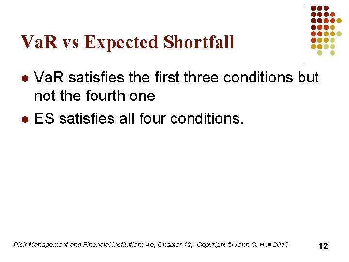
Va. R vs Expected Shortfall l l Va. R satisfies the first three conditions but not the fourth one ES satisfies all four conditions. Risk Management and Financial Institutions 4 e, Chapter 12, Copyright © John C. Hull 2015 12

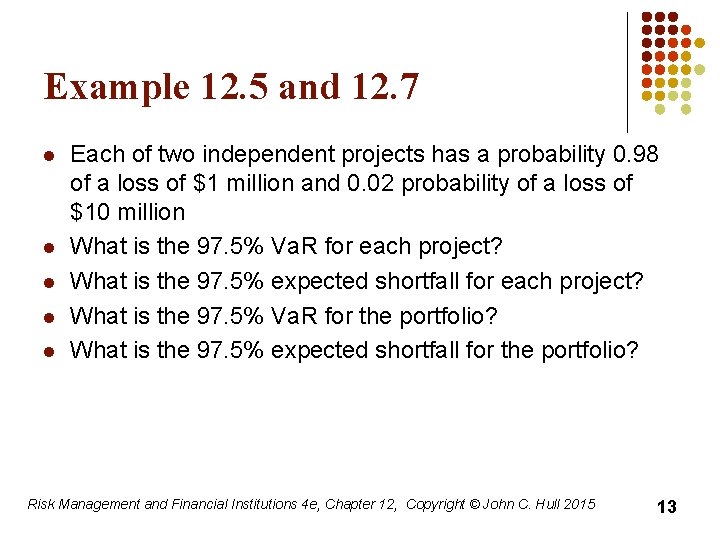
Example 12. 5 and 12. 7 l l l Each of two independent projects has a probability 0. 98 of a loss of $1 million and 0. 02 probability of a loss of $10 million What is the 97. 5% Va. R for each project? What is the 97. 5% expected shortfall for each project? What is the 97. 5% Va. R for the portfolio? What is the 97. 5% expected shortfall for the portfolio? Risk Management and Financial Institutions 4 e, Chapter 12, Copyright © John C. Hull 2015 13

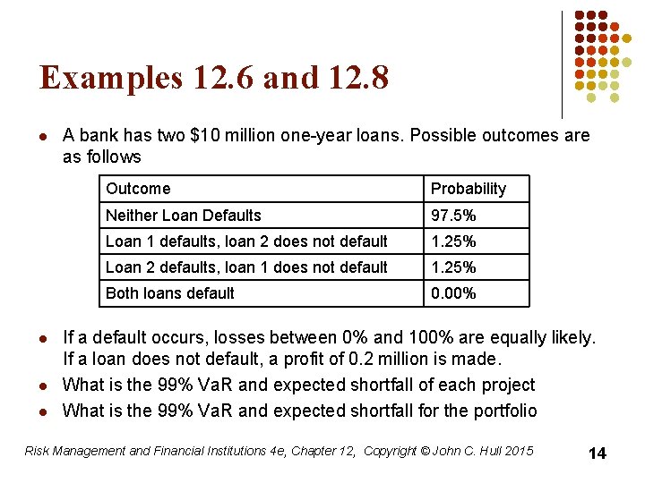
Examples 12. 6 and 12. 8 l l A bank has two $10 million one-year loans. Possible outcomes are as follows Outcome Probability Neither Loan Defaults 97. 5% Loan 1 defaults, loan 2 does not default 1. 25% Loan 2 defaults, loan 1 does not default 1. 25% Both loans default 0. 00% If a default occurs, losses between 0% and 100% are equally likely. If a loan does not default, a profit of 0. 2 million is made. What is the 99% Va. R and expected shortfall of each project What is the 99% Va. R and expected shortfall for the portfolio Risk Management and Financial Institutions 4 e, Chapter 12, Copyright © John C. Hull 2015 14

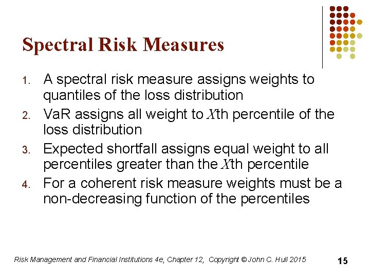
Spectral Risk Measures 1. 2. 3. 4. A spectral risk measure assigns weights to quantiles of the loss distribution Va. R assigns all weight to Xth percentile of the loss distribution Expected shortfall assigns equal weight to all percentiles greater than the Xth percentile For a coherent risk measure weights must be a non-decreasing function of the percentiles Risk Management and Financial Institutions 4 e, Chapter 12, Copyright © John C. Hull 2015 15

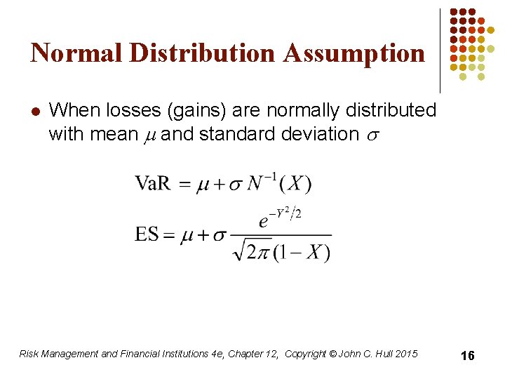
Normal Distribution Assumption l When losses (gains) are normally distributed with mean m and standard deviation s Risk Management and Financial Institutions 4 e, Chapter 12, Copyright © John C. Hull 2015 16

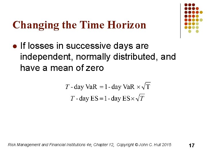
Changing the Time Horizon l If losses in successive days are independent, normally distributed, and have a mean of zero Risk Management and Financial Institutions 4 e, Chapter 12, Copyright © John C. Hull 2015 17

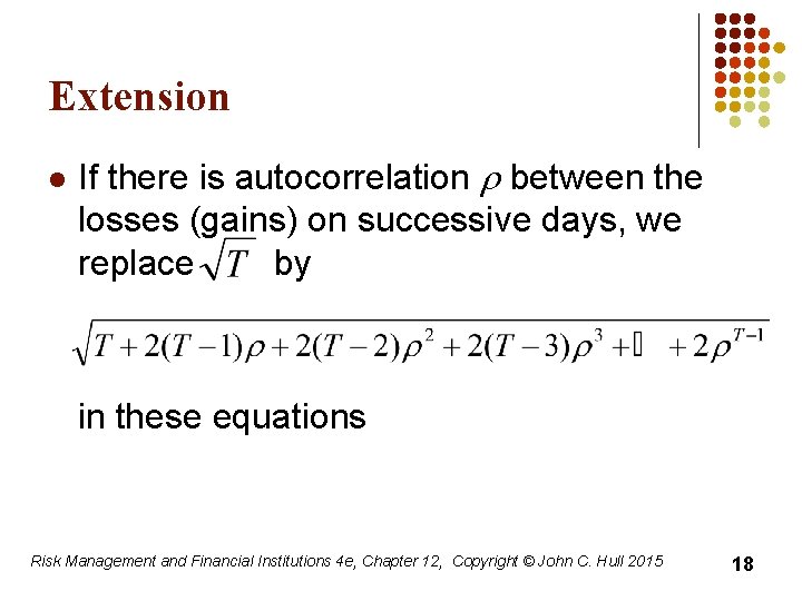
Extension l If there is autocorrelation r between the losses (gains) on successive days, we replace by in these equations Risk Management and Financial Institutions 4 e, Chapter 12, Copyright © John C. Hull 2015 18

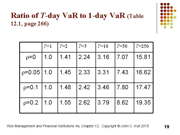
Ratio of T-day Va. R to 1 -day Va. R (Table 12. 1, page 266) T=1 T=2 T=5 T=10 T=50 T=250 1. 41 2. 24 3. 16 7. 07 15. 81 r=0. 05 1. 0 1. 45 2. 33 3. 31 7. 43 16. 62 r=0. 1 1. 0 1. 48 2. 42 3. 46 7. 80 17. 47 r=0. 2 1. 0 1. 55 2. 62 3. 79 8. 62 19. 35 r=0 Risk Management and Financial Institutions 4 e, Chapter 12, Copyright © John C. Hull 2015 19

Choice of Va. R Parameters l l l Time horizon should depend on how quickly portfolio can be unwound. Regulators are planning to move toward a system where ES is used and the time horizon depends on liquidity. (See Fundamental Review of the Trading Book) Confidence level depends on objectives. Regulators use 99% for market risk and 99. 9% for credit/operational risk. A bank wanting to maintain a AA credit rating might use confidence levels as high as 99. 97% for internal calculations. Risk Management and Financial Institutions 4 e, Chapter 12, Copyright © John C. Hull 2015 20

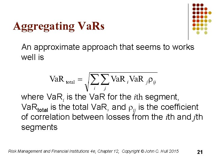
Aggregating Va. Rs An approximate approach that seems to works well is where Va. Ri is the Va. R for the ith segment, Va. Rtotal is the total Va. R, and rij is the coefficient of correlation between losses from the ith and jth segments Risk Management and Financial Institutions 4 e, Chapter 12, Copyright © John C. Hull 2015 21

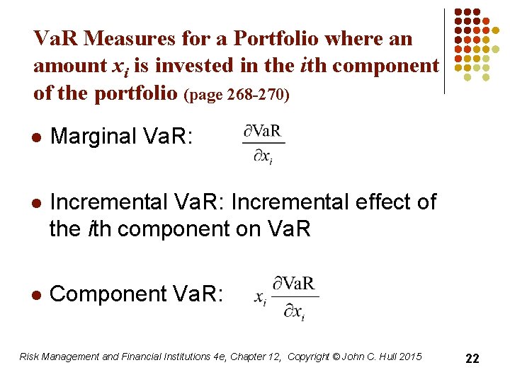
Va. R Measures for a Portfolio where an amount xi is invested in the ith component of the portfolio (page 268 -270) l Marginal Va. R: l Incremental Va. R: Incremental effect of the ith component on Va. R l Component Va. R: Risk Management and Financial Institutions 4 e, Chapter 12, Copyright © John C. Hull 2015 22

Properties of Component Va. R l l l The component Va. R is approximately the same as the incremental Va. R The total Va. R is the sum of the component Va. R’s (Euler’s theorem) The component Va. R therefore provides a sensible way of allocating Va. R to different activities Risk Management and Financial Institutions 4 e, Chapter 12, Copyright © John C. Hull 2015 23

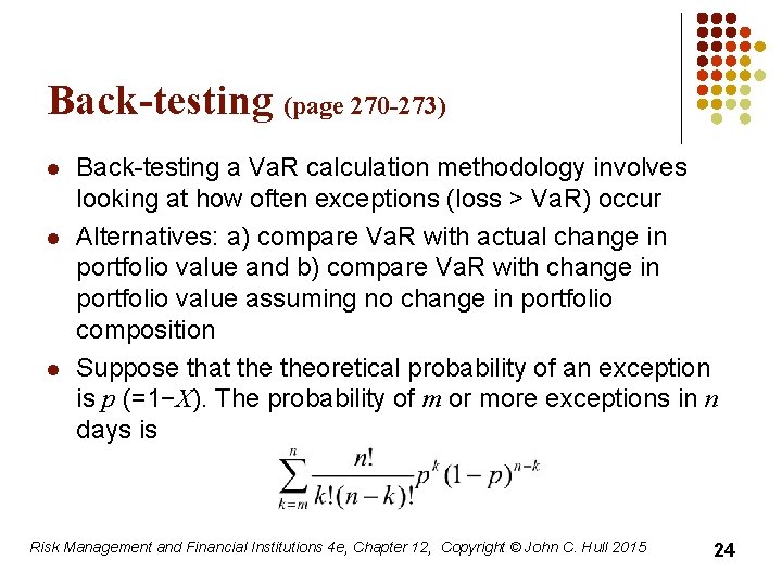
Back-testing (page 270 -273) l l l Back-testing a Va. R calculation methodology involves looking at how often exceptions (loss > Va. R) occur Alternatives: a) compare Va. R with actual change in portfolio value and b) compare Va. R with change in portfolio value assuming no change in portfolio composition Suppose that theoretical probability of an exception is p (=1−X). The probability of m or more exceptions in n days is Risk Management and Financial Institutions 4 e, Chapter 12, Copyright © John C. Hull 2015 24

Bunching l l Bunching occurs when exceptions are not evenly spread throughout the back testing period Statistical tests for bunching have been developed by Christoffersen (See page 200) Risk Management and Financial Institutions 4 e, Chapter 12, Copyright © John C. Hull 2015 25