V Latin squares designs LS V A Design

V. Latin squares designs (LS) V. A Design of Latin squares V. B Indicator-variable models and estimation for a Latin square V. C Hypothesis testing using the ANOVA method for a Latin square V. D Diagnostic checking V. E Treatment differences V. F Design of sets of Latin squares V. G Hypothesis tests for sets of Latin squares Statistical Modelling Chapter V 1

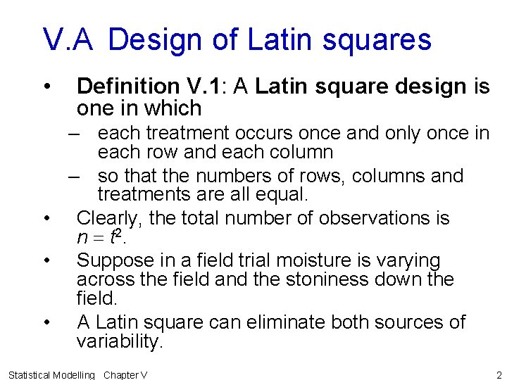
V. A Design of Latin squares • Definition V. 1: A Latin square design is one in which – each treatment occurs once and only once in each row and each column – so that the numbers of rows, columns and treatments are all equal. • Clearly, the total number of observations is n = t 2. • Suppose in a field trial moisture is varying across the field and the stoniness down the field. • A Latin square can eliminate both sources of variability. Statistical Modelling Chapter V 2

Example V. 1 Fertilizer experiment Statistical Modelling Chapter V 3

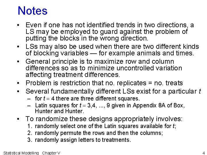
Notes • Even if one has not identified trends in two directions, a LS may be employed to guard against the problem of putting the blocks in the wrong direction. • LSs may also be used when there are two different kinds of blocking variables — for example animals and times. • General principle is to maximize row and column differences so as to minimize uncontrolled variation affecting treatment differences. • Problem is restriction that no. replicates = no. treats • Several fundamentally different LSs exist for a particular t – for t = 4 there are three different squares. – Latin squares for t = 3, 4, . . . , 9 given in Appendix 8 A of Box, Hunter and Hunter. • To randomize these designs appropriately involves: 1. randomly select one of the Latin squares available for t; 2. randomly permute the rows and then the columns; 3. randomly assign letters to treatments. Statistical Modelling Chapter V 4

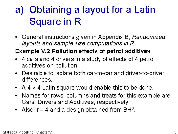
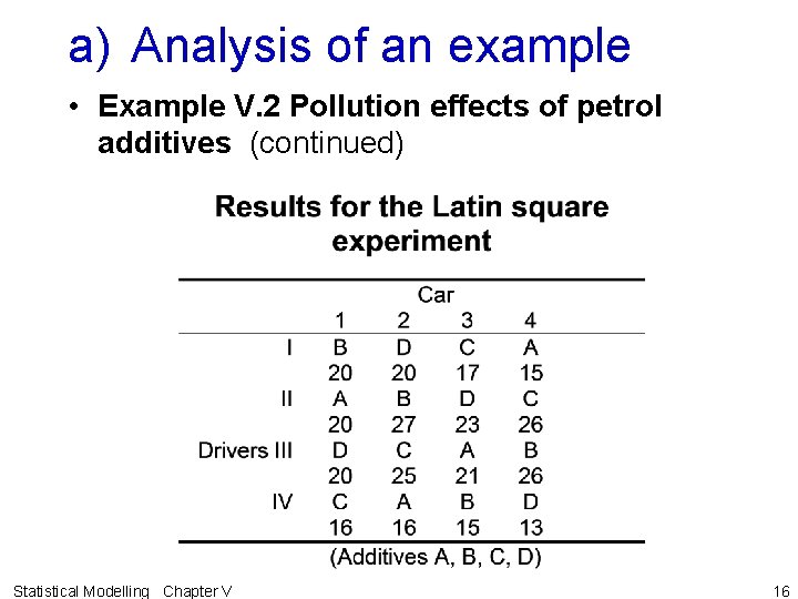
a) Obtaining a layout for a Latin Square in R • General instructions given in Appendix B, Randomized layouts and sample size computations in R. Example V. 2 Pollution effects of petrol additives • 4 cars and 4 drivers in a study of effects of 4 petrol additives on pollution. • Desirable to isolate both car-to-car and driver-to-driver differences. • A 4 4 Latin square would enable this to be done. • Names for rows, columns and treats for this example are Cars, Drivers and Additives, respectively. • Also, t = 4 and a design obtained from BH 2. Statistical Modelling Chapter V 5

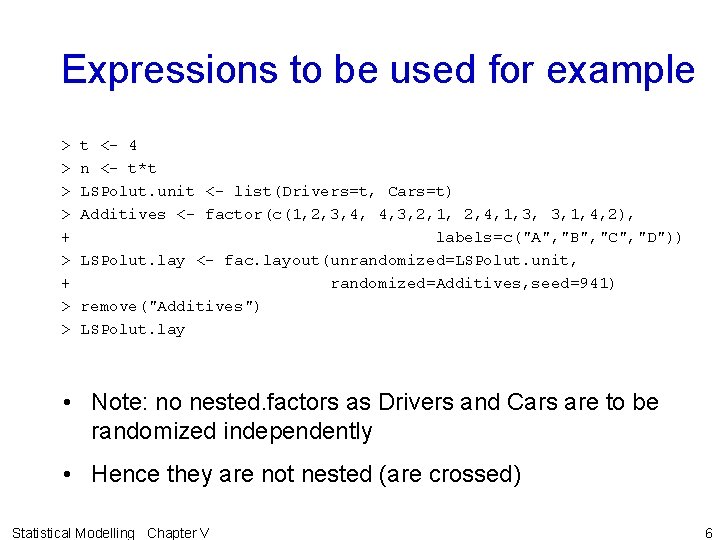
Expressions to be used for example > t <- 4 > n <- t*t > LSPolut. unit <- list(Drivers=t, Cars=t) > Additives <- factor(c(1, 2, 3, 4, 4, 3, 2, 1, 2, 4, 1, 3, 3, 1, 4, 2), + labels=c("A", "B", "C", "D")) > LSPolut. lay <- fac. layout(unrandomized=LSPolut. unit, + randomized=Additives, seed=941) > remove("Additives") > LSPolut. lay • Note: no nested. factors as Drivers and Cars are to be randomized independently • Hence they are not nested (are crossed) Statistical Modelling Chapter V 6

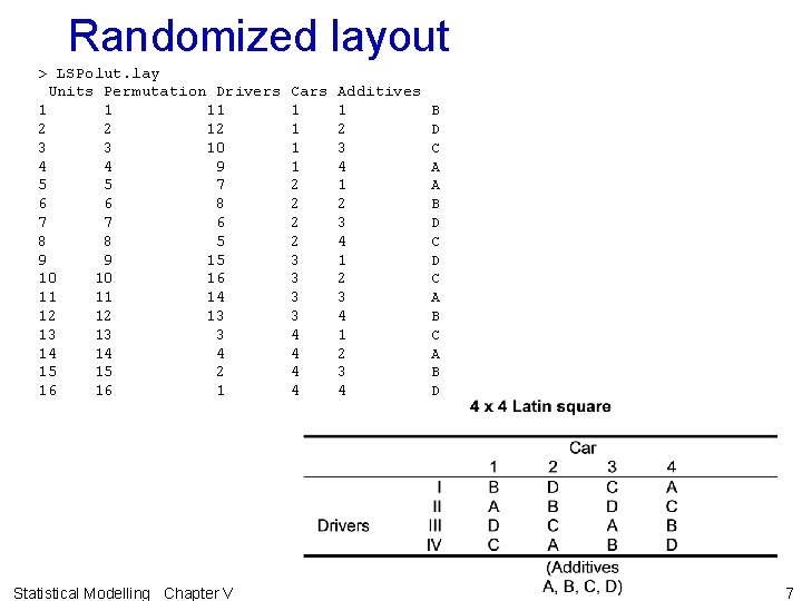
Randomized layout > LSPolut. lay Units Permutation Drivers Cars Additives 1 1 11 1 1 B 2 2 12 1 2 D 3 3 10 1 3 C 4 4 9 1 4 A 5 5 7 2 1 A 6 6 8 2 2 B 7 7 6 2 3 D 8 8 5 2 4 C 9 9 15 3 1 D 10 16 3 2 C 11 14 3 3 A 12 13 3 4 B 13 3 4 1 C 14 4 4 2 A 15 2 4 3 B 16 1 4 4 D Statistical Modelling Chapter V 7

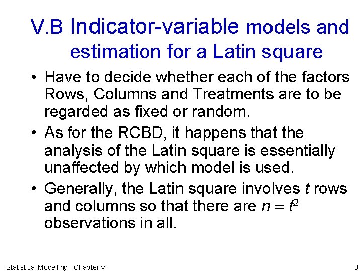
V. B Indicator-variable models and estimation for a Latin square • Have to decide whether each of the factors Rows, Columns and Treatments are to be regarded as fixed or random. • As for the RCBD, it happens that the analysis of the Latin square is essentially unaffected by which model is used. • Generally, the Latin square involves t rows and columns so that there are n = t 2 observations in all. Statistical Modelling Chapter V 8

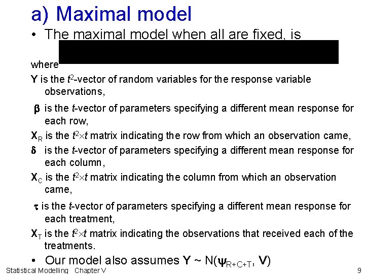
a) Maximal model • The maximal model when all are fixed, is where Y is the t 2 -vector of random variables for the response variable observations, b is the t-vector of parameters specifying a different mean response for each row, XR is the t 2 t matrix indicating the row from which an observation came, d is the t-vector of parameters specifying a different mean response for each column, XC is the t 2 t matrix indicating the column from which an observation came, t is the t-vector of parameters specifying a different mean response for each treatment, XT is the t 2 t matrix indicating the observations that received each of the treatments. • Our model also assumes Y ~ N(y. R+C+T, V) Statistical Modelling Chapter V 9

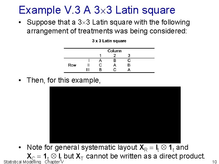
Example V. 3 A 3 3 Latin square • Suppose that a 3 3 Latin square with the following arrangement of treatments was being considered: • Then, for this example, • Note for general systematic layout XR = It 1 t and XC = 1 t It but XT cannot be written as a direct product. Statistical Modelling Chapter V 10

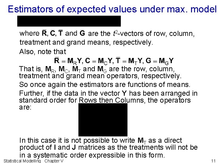
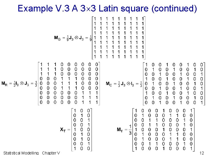
Estimators of expected values under max. model are the t 2 -vectors of row, column, treatment and grand means, respectively. Also, note that That is, MR, MC, MT and MG are the row, column, treatment and grand mean operators, respectively. So once again the estimators are functions of means. Further, if the data in the vector Y has been arranged in standard order for Rows then Columns, the operators are: In this case it is not possible to write MT as a direct product of I and J matrices as the treatments will not be in a systematic order expressible in this form. Statistical Modelling Chapter V 11

Example V. 3 A 3 3 Latin square (continued) Statistical Modelling Chapter V 12

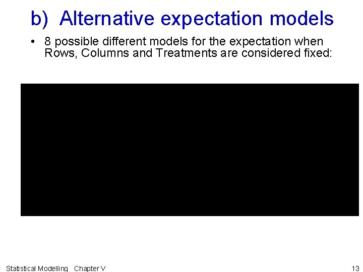
b) Alternative expectation models • 8 possible different models for the expectation when Rows, Columns and Treatments are considered fixed: Statistical Modelling Chapter V 13

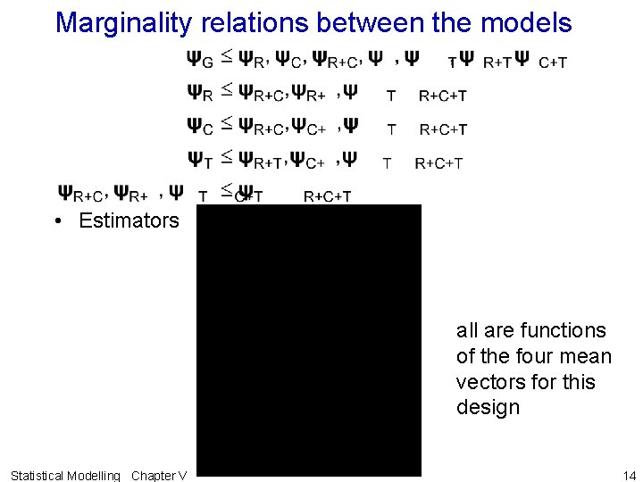
Marginality relations between the models • Estimators all are functions of the four mean vectors for this design Statistical Modelling Chapter V 14

V. C Hypothesis testing using the ANOVA method for a Latin square • An ANOVA will be used to choose between the 8 alternative expectation models for a Latin square. Statistical Modelling Chapter V 15

a) Analysis of an example • Example V. 2 Pollution effects of petrol additives (continued) Statistical Modelling Chapter V 16

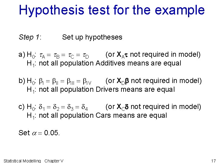
Hypothesis test for the example Step 1: Set up hypotheses a) H 0: t. A = t. B = t. C = t. D (or XAt not required in model) H 1: not all population Additives means are equal b) H 0: b. I = b. III = b. IV (or XDb not required in model) H 1: not all population Drivers means are equal c) H 0: d 1 = d 2 = d 3 = d 4 (or XCd not required in model) H 1: not all population Cars means are equal Set a = 0. 05. Statistical Modelling Chapter V 17

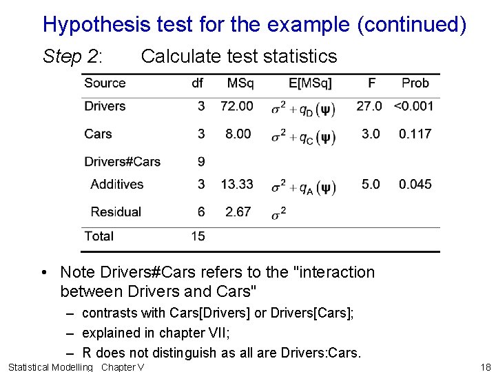
Hypothesis test for the example (continued) Step 2: Calculate test statistics • Note Drivers#Cars refers to the "interaction between Drivers and Cars" – contrasts with Cars[Drivers] or Drivers[Cars]; – explained in chapter VII; – R does not distinguish as all are Drivers: Cars. Statistical Modelling Chapter V 18

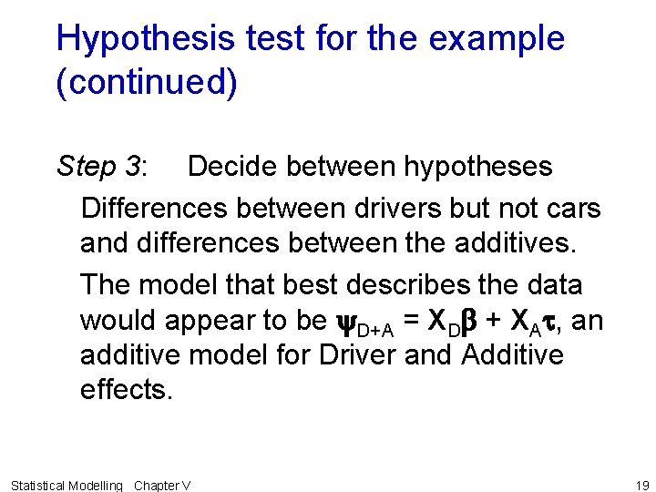
Hypothesis test for the example (continued) Step 3: Decide between hypotheses Differences between drivers but not cars and differences between the additives. The model that best describes the data would appear to be y. D+A = XDb + XAt, an additive model for Driver and Additive effects. Statistical Modelling Chapter V 19

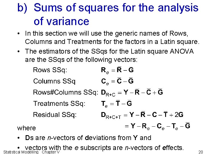
b) Sums of squares for the analysis of variance • In this section we will use the generic names of Rows, Columns and Treatments for the factors in a Latin square. • The estimators of the SSqs for the Latin square ANOVA are the SSqs of the following vectors: where • Ds are n-vectors of deviations from Y and • vectors with the e subscripts are n-vectors of effects. Statistical Modelling Chapter V 20

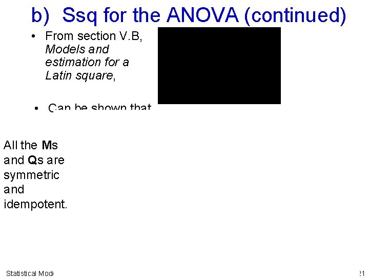
b) Ssq for the ANOVA (continued) • From section V. B, Models and estimation for a Latin square, • Can be shown that All the Ms and Qs are symmetric and idempotent. Statistical Modelling Chapter V 21

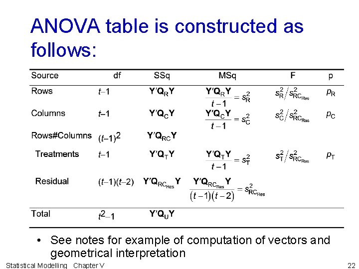
ANOVA table is constructed as follows: • See notes for example of computation of vectors and geometrical interpretation Statistical Modelling Chapter V 22

c) Expected mean squares • To justify our choice of test statistics, we want to work out the E[MSq]s in the ANOVA table under the 8 alternative expectation models. • However, to save space work out E[MSq]s under the maximal model and identify which terms in E[MSq]s go to zero under alternative models. Statistical Modelling Chapter V 24

E[MSq]s with fixed Rows and Columns effects • • • Given the expressions in the above table, the population means of the mean squares could be computed if knew the bis, djs, tks and s 2. Each of q. R(y), q. C(y) and q. T(y) equal 0 when the terms XRb, XCd and XTt, respectively, removed from the model. Hence a significant F value for a line indicates that the corresponding term should be included in the model. Statistical Modelling Chapter V 25

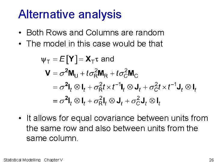
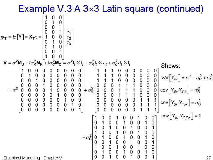
Alternative analysis • Both Rows and Columns are random • The model in this case would be that • It allows for equal covariance between units from the same row and also between units from the same column. Statistical Modelling Chapter V 26

Example V. 3 A 3 3 Latin square (continued) Shows: Statistical Modelling Chapter V 27

E[MSq]s under alternative model • Alternative expectation model is y. G = XGm and under this model q. T(y) = 0. • Alternative variance models involve setting and/or and this will result in the one(s) set to zero being dropped from the expected mean square. • This exactly parallels what happens when both are fixed. Statistical Modelling Chapter V 28

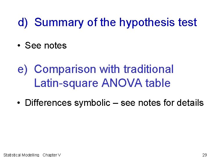
d) Summary of the hypothesis test • See notes e) Comparison with traditional Latin-square ANOVA table • Differences symbolic – see notes for details Statistical Modelling Chapter V 29

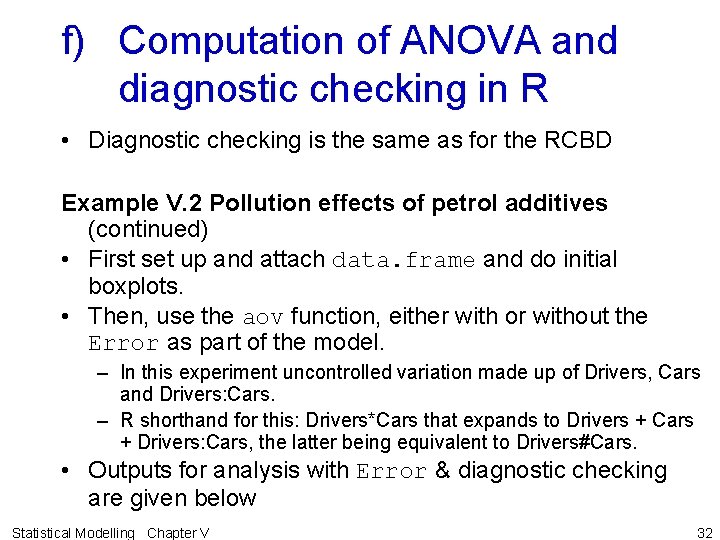
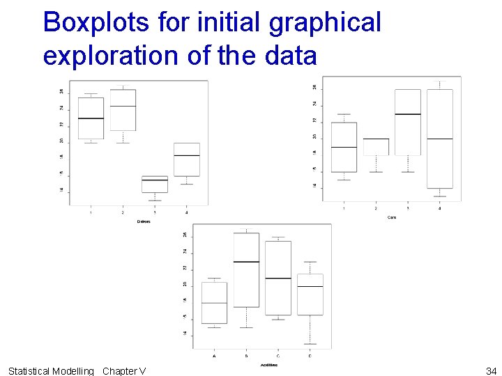
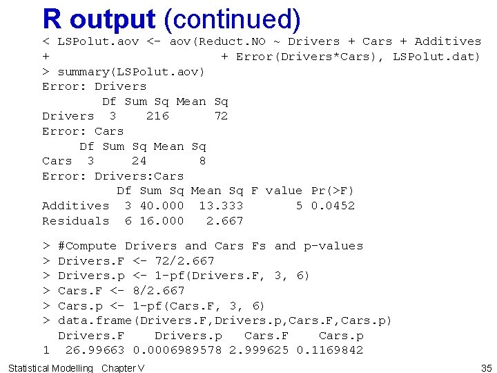
f) Computation of ANOVA and diagnostic checking in R • Diagnostic checking is the same as for the RCBD Example V. 2 Pollution effects of petrol additives (continued) • First set up and attach data. frame and do initial boxplots. • Then, use the aov function, either with or without the Error as part of the model. – In this experiment uncontrolled variation made up of Drivers, Cars and Drivers: Cars. – R shorthand for this: Drivers*Cars that expands to Drivers + Cars + Drivers: Cars, the latter being equivalent to Drivers#Cars. • Outputs for analysis with Error & diagnostic checking are given below Statistical Modelling Chapter V 32

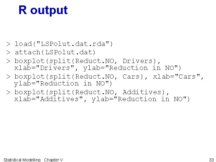
R output > load("LSPolut. dat. rda") > attach(LSPolut. dat) > boxplot(split(Reduct. NO, Drivers), xlab="Drivers", ylab="Reduction in NO") > boxplot(split(Reduct. NO, Cars), xlab="Cars", ylab="Reduction in NO") > boxplot(split(Reduct. NO, Additives), xlab="Additives", ylab="Reduction in NO") Statistical Modelling Chapter V 33

Boxplots for initial graphical exploration of the data Statistical Modelling Chapter V 34

R output (continued) < LSPolut. aov <- aov(Reduct. NO ~ Drivers + Cars + Additives + + Error(Drivers*Cars), LSPolut. dat) > summary(LSPolut. aov) Error: Drivers Df Sum Sq Mean Sq Drivers 3 216 72 Error: Cars Df Sum Sq Mean Sq Cars 3 24 8 Error: Drivers: Cars Df Sum Sq Mean Sq F value Pr(>F) Additives 3 40. 000 13. 333 5 0. 0452 Residuals 6 16. 000 2. 667 > #Compute Drivers and Cars Fs and p-values > Drivers. F <- 72/2. 667 > Drivers. p <- 1 -pf(Drivers. F, 3, 6) > Cars. F <- 8/2. 667 > Cars. p <- 1 -pf(Cars. F, 3, 6) > data. frame(Drivers. F, Drivers. p, Cars. F, Cars. p) Drivers. F Drivers. p Cars. F Cars. p 1 26. 99663 0. 0006989578 2. 999625 0. 1169842 Statistical Modelling Chapter V 35

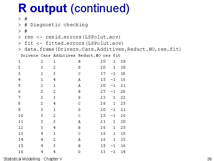
R output (continued) > # Diagnostic checking > # > res <- resid. errors(LSPolut. aov) > fit <- fitted. errors(LSPolut. aov) > data. frame(Drivers, Cars, Additives, Reduct. NO, res, fit) Drivers Cars Additives Reduct. NO res fit 1 1 1 B 20 1 19 2 1 2 D 20 1 19 3 1 3 C 17 -1 18 4 1 4 A 15 -1 16 5 2 1 A 20 -1 21 6 2 2 B 27 -1 28 7 2 3 D 23 1 22 8 2 4 C 26 1 25 9 3 1 D 20 -1 21 10 3 2 C 25 -1 26 11 3 3 A 21 1 20 12 3 4 B 26 1 25 13 4 1 C 16 1 15 14 4 2 A 16 1 15 15 4 3 B 15 -1 16 16 4 4 D 13 -1 14 Statistical Modelling Chapter V 36

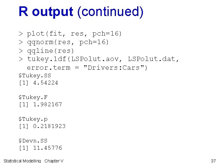
R output (continued) > plot(fit, res, pch=16) > qqnorm(res, pch=16) > qqline(res) > tukey. 1 df(LSPolut. aov, LSPolut. dat, error. term = "Drivers: Cars") $Tukey. SS [1] 4. 54224 $Tukey. F [1] 1. 982167 $Tukey. p [1] 0. 2181923 $Devn. SS [1] 11. 45776 Statistical Modelling Chapter V 37

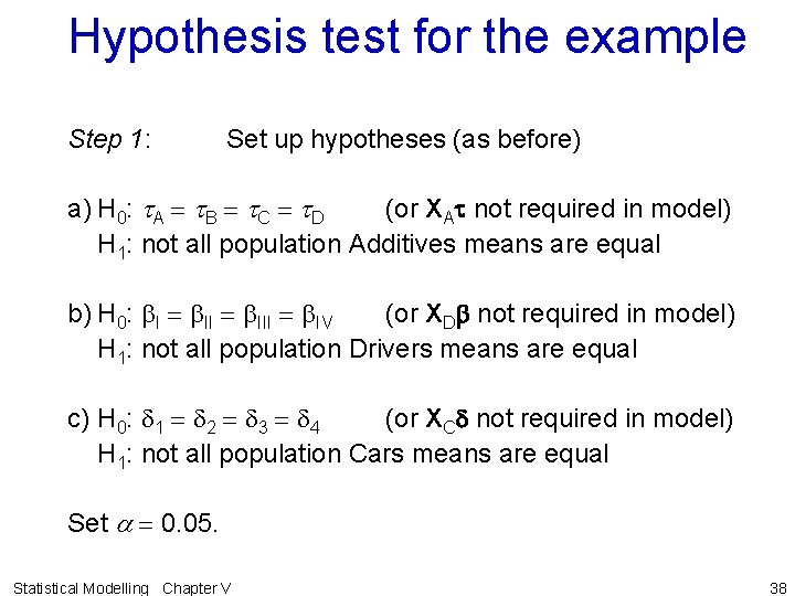
Hypothesis test for the example Step 1: Set up hypotheses (as before) a) H 0: t. A = t. B = t. C = t. D (or XAt not required in model) H 1: not all population Additives means are equal b) H 0: b. I = b. III = b. IV (or XDb not required in model) H 1: not all population Drivers means are equal c) H 0: d 1 = d 2 = d 3 = d 4 (or XCd not required in model) H 1: not all population Cars means are equal Set a = 0. 05. Statistical Modelling Chapter V 38

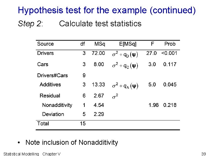
Hypothesis test for the example (continued) Step 2: Calculate test statistics • Note inclusion of Nonadditivity Statistical Modelling Chapter V 39

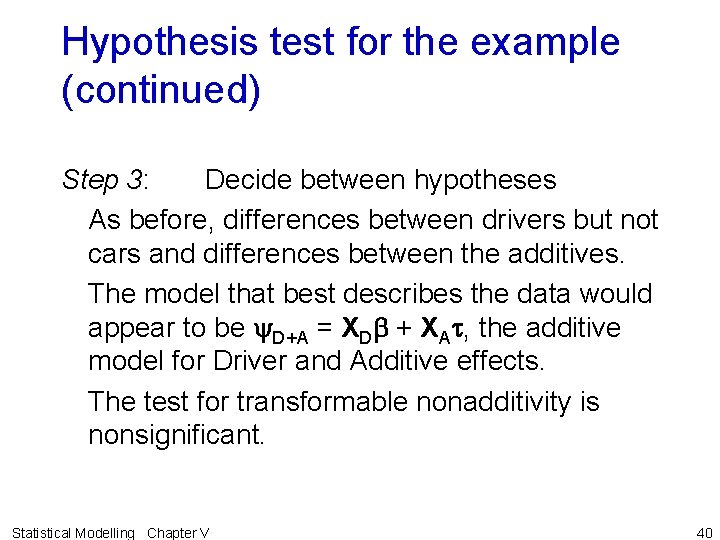
Hypothesis test for the example (continued) Step 3: Decide between hypotheses As before, differences between drivers but not cars and differences between the additives. The model that best describes the data would appear to be y. D+A = XDb + XAt, the additive model for Driver and Additive effects. The test for transformable nonadditivity is nonsignificant. Statistical Modelling Chapter V 40

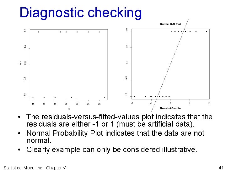
Diagnostic checking • The residuals-versus-fitted-values plot indicates that the residuals are either -1 or 1 (must be artificial data). • Normal Probability Plot indicates that the data are not normal. • Clearly example can only be considered illustrative. Statistical Modelling Chapter V 41

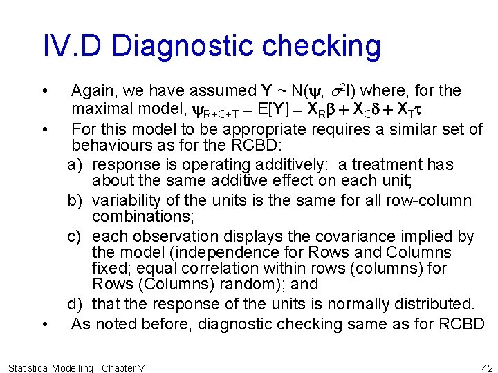
IV. D Diagnostic checking • • • Again, we have assumed Y ~ N(y, s 2 I) where, for the maximal model, y. R+C+T = E[Y] = XRb + XCd + XTt For this model to be appropriate requires a similar set of behaviours as for the RCBD: a) response is operating additively: a treatment has about the same additive effect on each unit; b) variability of the units is the same for all row-column combinations; c) each observation displays the covariance implied by the model (independence for Rows and Columns fixed; equal correlation within rows (columns) for Rows (Columns) random); and d) that the response of the units is normally distributed. As noted before, diagnostic checking same as for RCBD Statistical Modelling Chapter V 42

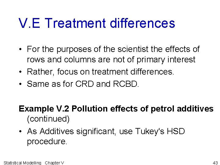
V. E Treatment differences • For the purposes of the scientist the effects of rows and columns are not of primary interest • Rather, focus on treatment differences. • Same as for CRD and RCBD. Example V. 2 Pollution effects of petrol additives (continued) • As Additives significant, use Tukey's HSD procedure. Statistical Modelling Chapter V 43

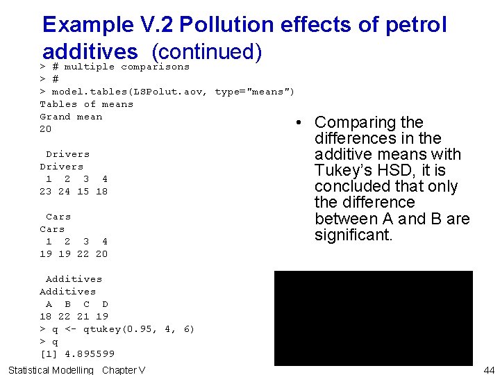
Example V. 2 Pollution effects of petrol additives (continued) > # multiple comparisons > # > model. tables(LSPolut. aov, type="means") Tables of means Grand mean 20 Drivers 1 2 3 4 23 24 15 18 Cars 1 2 3 4 19 19 22 20 • Comparing the differences in the additive means with Tukey’s HSD, it is concluded that only the difference between A and B are significant. Additives A B C D 18 22 21 19 > q <- qtukey(0. 95, 4, 6) > q [1] 4. 895599 Statistical Modelling Chapter V 44

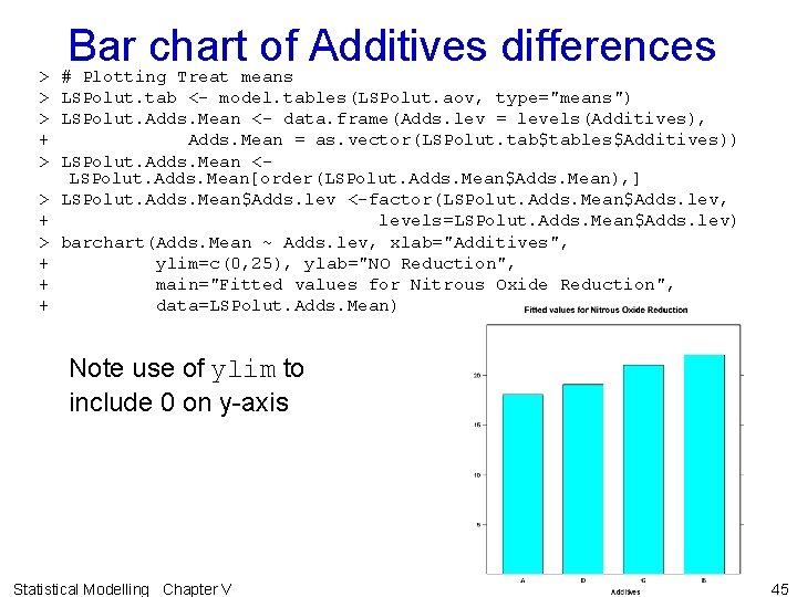
Bar chart of Additives differences > # Plotting Treat means > LSPolut. tab <- model. tables(LSPolut. aov, type="means") > LSPolut. Adds. Mean <- data. frame(Adds. lev = levels(Additives), + Adds. Mean = as. vector(LSPolut. tab$tables$Additives)) > LSPolut. Adds. Mean <- LSPolut. Adds. Mean[order(LSPolut. Adds. Mean$Adds. Mean), ] > LSPolut. Adds. Mean$Adds. lev <-factor(LSPolut. Adds. Mean$Adds. lev, + levels=LSPolut. Adds. Mean$Adds. lev) > barchart(Adds. Mean ~ Adds. lev, xlab="Additives", + ylim=c(0, 25), ylab="NO Reduction", + main="Fitted values for Nitrous Oxide Reduction", + data=LSPolut. Adds. Mean) Note use of ylim to include 0 on y-axis Statistical Modelling Chapter V 45

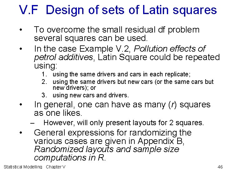
V. F Design of sets of Latin squares • • To overcome the small residual df problem several squares can be used. In the case Example V. 2, Pollution effects of petrol additives, Latin Square could be repeated using: 1. using the same drivers and cars in each replicate; 2. using the same drivers but new cars (or the same cars but new drivers); or 3. using new cars and drivers. • In general, one can have as many (r) squares as one likes. – • However, will only present layouts for 2 squares. General expressions for randomizing the various cases are given in Appendix B, Randomized layouts and sample size computations in R. Statistical Modelling Chapter V 46

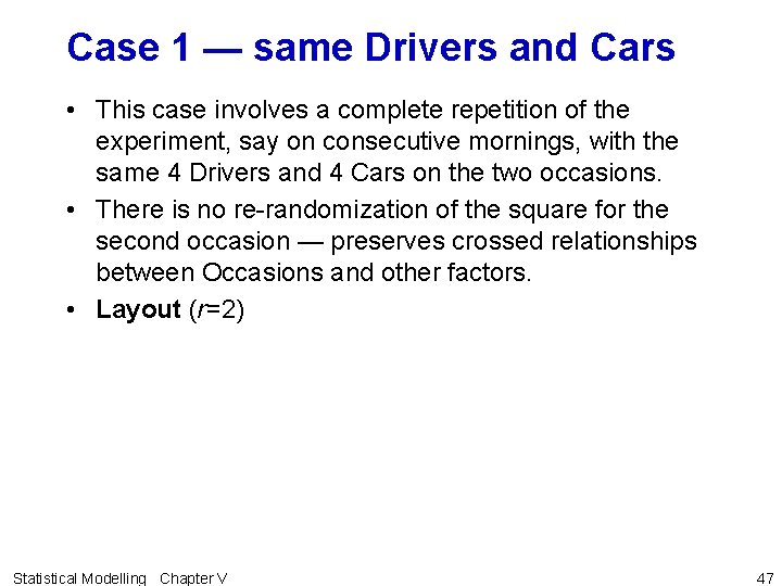
Case 1 — same Drivers and Cars • This case involves a complete repetition of the experiment, say on consecutive mornings, with the same 4 Drivers and 4 Cars on the two occasions. • There is no re-randomization of the square for the second occasion — preserves crossed relationships between Occasions and other factors. • Layout (r=2) Statistical Modelling Chapter V 47

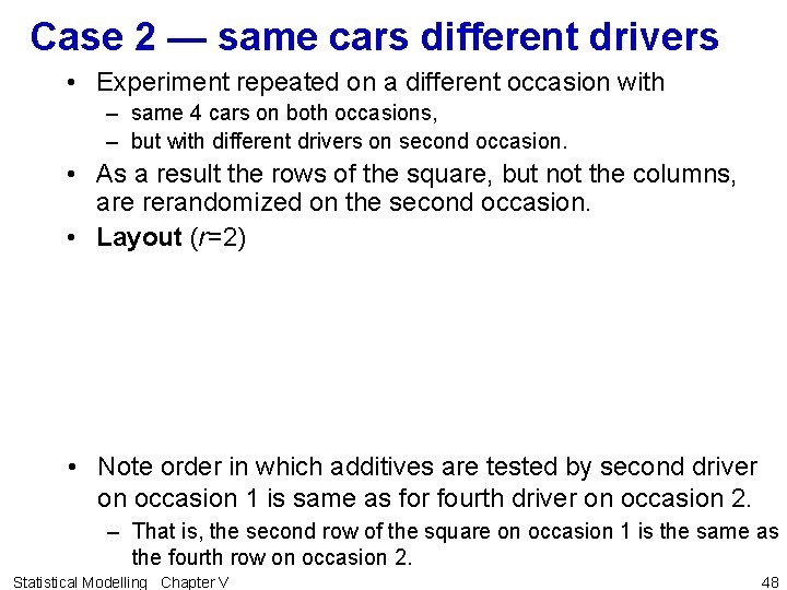
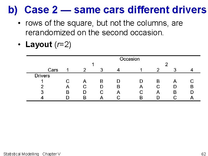
Case 2 — same cars different drivers • Experiment repeated on a different occasion with – same 4 cars on both occasions, – but with different drivers on second occasion. • As a result the rows of the square, but not the columns, are rerandomized on the second occasion. • Layout (r=2) • Note order in which additives are tested by second driver on occasion 1 is same as for fourth driver on occasion 2. – That is, the second row of the square on occasion 1 is the same as the fourth row on occasion 2. Statistical Modelling Chapter V 48

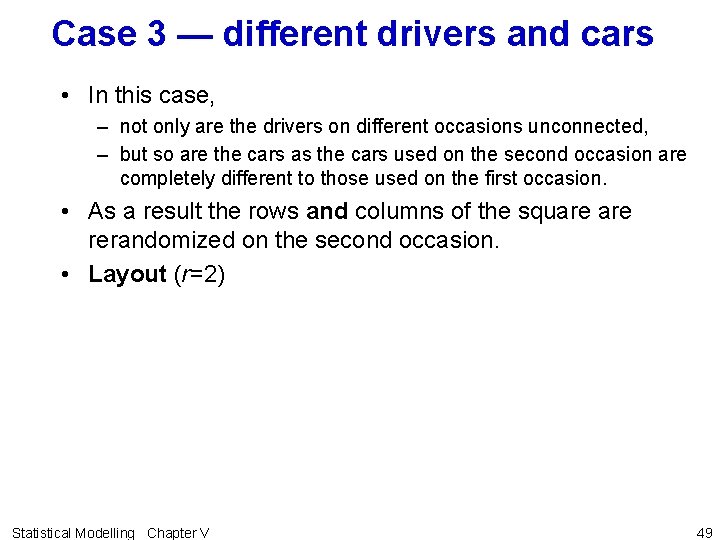
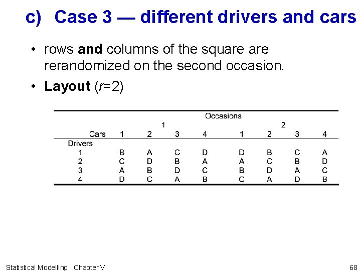
Case 3 — different drivers and cars • In this case, – not only are the drivers on different occasions unconnected, – but so are the cars as the cars used on the second occasion are completely different to those used on the first occasion. • As a result the rows and columns of the square rerandomized on the second occasion. • Layout (r=2) Statistical Modelling Chapter V 49

V. G Hypothesis tests for sets of Latin squares • In previous section discussed the use of several squares to overcome the residual df problem. – • e. g. 4 4 Latin square has 6 (< 10) Residual df Gave 3 cases for Example V. 2, Pollution effects of petrol additives: 1. 2. 3. • • Shall determine ANOVA for each of these cases. In determining the E[MSq]s will be assumed that – – • using the same drivers and cars in each replicate; using the same drivers but new cars (or the same cars but new drivers); or using new cars and drivers. unrandomized factors are to be classified as random factors randomized factors as fixed factors. While layouts were for 2 squares will give DF for the general case of r squares. Statistical Modelling Chapter V 50

a) Case 1 — same Drivers and Cars • no re-randomization of the square for the second occasion • Layout (r=2) Statistical Modelling Chapter V 51

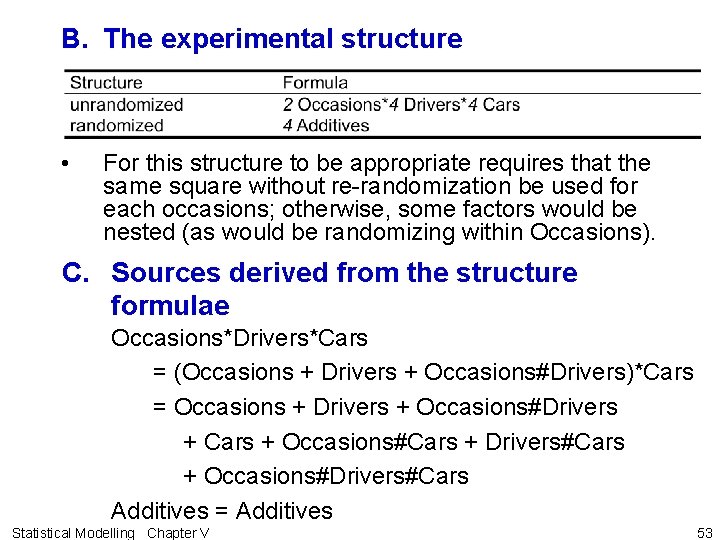
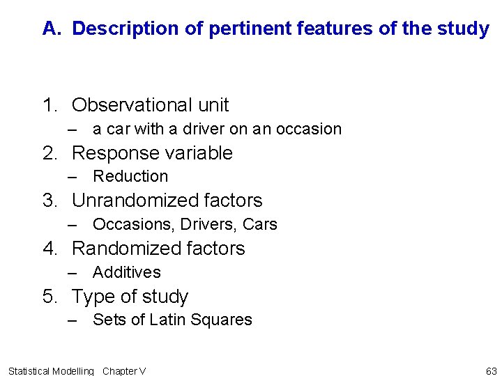
A. Description of pertinent features of the study 1. Observational unit – a car with a driver on an occasion 2. Response variable – Reduction 3. Unrandomized factors – Occasions, Drivers, Cars 4. Randomized factors – Additives 5. Type of study – Sets of Latin Squares Statistical Modelling Chapter V 52

B. The experimental structure • For this structure to be appropriate requires that the same square without re-randomization be used for each occasions; otherwise, some factors would be nested (as would be randomizing within Occasions). C. Sources derived from the structure formulae Occasions*Drivers*Cars = (Occasions + Drivers + Occasions#Drivers)*Cars = Occasions + Drivers + Occasions#Drivers + Cars + Occasions#Cars + Drivers#Cars + Occasions#Drivers#Cars Additives = Additives Statistical Modelling Chapter V 53

D. Degrees of freedom and sums of squares • Hasse diagrams, with degrees of freedom, for this study are: Statistical Modelling Chapter V 54

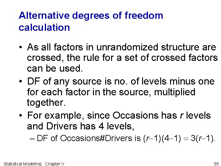
Alternative degrees of freedom calculation • As all factors in unrandomized structure are crossed, the rule for a set of crossed factors can be used. • DF of any source is no. of levels minus one for each factor in the source, multiplied together. • For example, since Occasions has r levels and Drivers has 4 levels, – DF of Occasions#Drivers is (r-1)(4 -1) = 3(r-1). Statistical Modelling Chapter V 55

Hasse diagrams, with M and Q matrices Statistical Modelling Chapter V 56

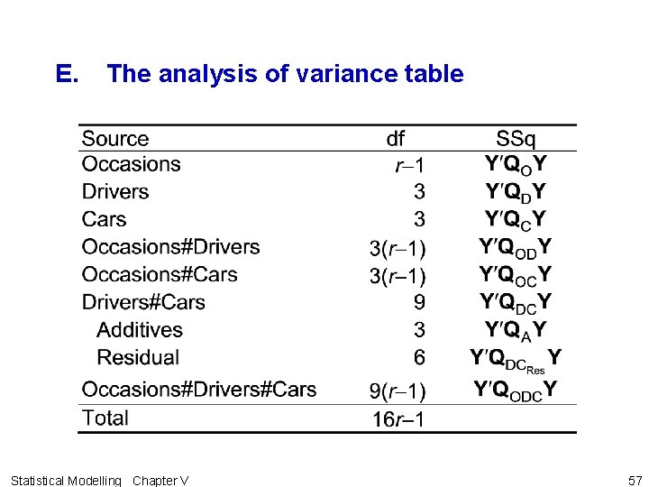
E. The analysis of variance table Statistical Modelling Chapter V 57

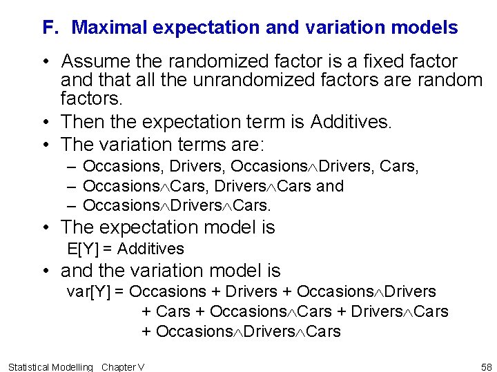
F. Maximal expectation and variation models • Assume the randomized factor is a fixed factor and that all the unrandomized factors are random factors. • Then the expectation term is Additives. • The variation terms are: – Occasions, Drivers, Occasions Drivers, Cars, – Occasions Cars, Drivers Cars and – Occasions Drivers Cars. • The expectation model is E[Y] = Additives • and the variation model is var[Y] = Occasions + Drivers + Occasions Drivers + Cars + Occasions Cars + Drivers Cars + Occasions Drivers Cars Statistical Modelling Chapter V 58

G. The expected mean squares • The Hasse diagram, with contributions to E[MSq]s, for the unrandomized factors in this study is: • The single randomized factor Additive will contribute q. A(y) to the E[MSq] for its source. Statistical Modelling Chapter V 59

ANOVA table with E[MSq] • Hypothesis tests for Additive, Occ#Drivers and Occ#Cars straightforward. • Tests for Occ, Drivers and Cars are more difficult. – For example, to test Occ, need ratio of 2 sums of MSqs. – DF a problem Statistical Modelling Chapter V 60

b) Case 2 — same cars different drivers • rows of the square, but not the columns, are rerandomized on the second occasion. • Layout (r=2) Statistical Modelling Chapter V 62

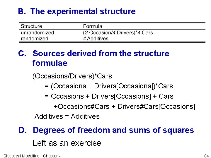
A. Description of pertinent features of the study 1. Observational unit – a car with a driver on an occasion 2. Response variable – Reduction 3. Unrandomized factors – Occasions, Drivers, Cars 4. Randomized factors – Additives 5. Type of study – Sets of Latin Squares Statistical Modelling Chapter V 63

B. The experimental structure C. Sources derived from the structure formulae (Occasions/Drivers)*Cars = (Occasions + Drivers[Occasions])*Cars = Occasions + Drivers[Occasions] + Cars +Occasions#Cars + Drivers#Cars[Occasions] Additives = Additives D. Degrees of freedom and sums of squares Left as an exercise Statistical Modelling Chapter V 64

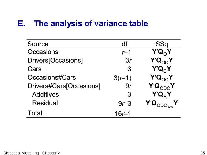
E. The analysis of variance table Statistical Modelling Chapter V 65

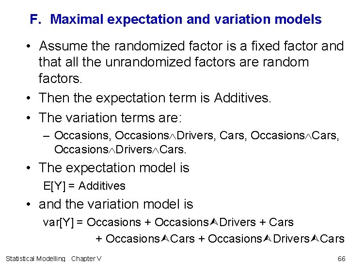
F. Maximal expectation and variation models • Assume the randomized factor is a fixed factor and that all the unrandomized factors are random factors. • Then the expectation term is Additives. • The variation terms are: – Occasions, Occasions Drivers, Cars, Occasions Cars, Occasions Drivers Cars. • The expectation model is E[Y] = Additives • and the variation model is var[Y] = Occasions + Occasions Drivers + Cars + Occasions Drivers Cars Statistical Modelling Chapter V 66

G. The expected mean squares • The Hasse diagram, with contributions to E[MSq]s, for the unrandomized factors in this study is left as an exercise. • The single randomized factor Additive will contribute q. A(y) to the E[MSq] for its source. ANOVA table with E[MSq] • Hypothesis tests for Drivers[Occasions], Cars, Occasions#Cars and Additives are straightforward • The test for Occasions is more difficult. Statistical Modelling Chapter V 67

c) Case 3 — different drivers and cars • rows and columns of the square rerandomized on the second occasion. • Layout (r=2) Statistical Modelling Chapter V 68

A. Description of pertinent features of the study 1. Observational unit – a car with a driver on an occasion 2. Response variable – Reduction 3. Unrandomized factors – Occasions, Drivers, Cars 4. Randomized factors – Additives 5. Type of study – Sets of Latin Squares Statistical Modelling Chapter V 69

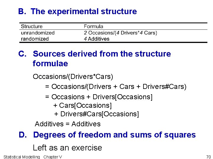
B. The experimental structure C. Sources derived from the structure formulae Occasions/(Drivers*Cars) = Occasions/(Drivers + Cars + Drivers#Cars) = Occasions + Drivers[Occasions] + Cars[Occasions] + Drivers#Cars[Occasions] Additives = Additives D. Degrees of freedom and sums of squares Left as an exercise Statistical Modelling Chapter V 70

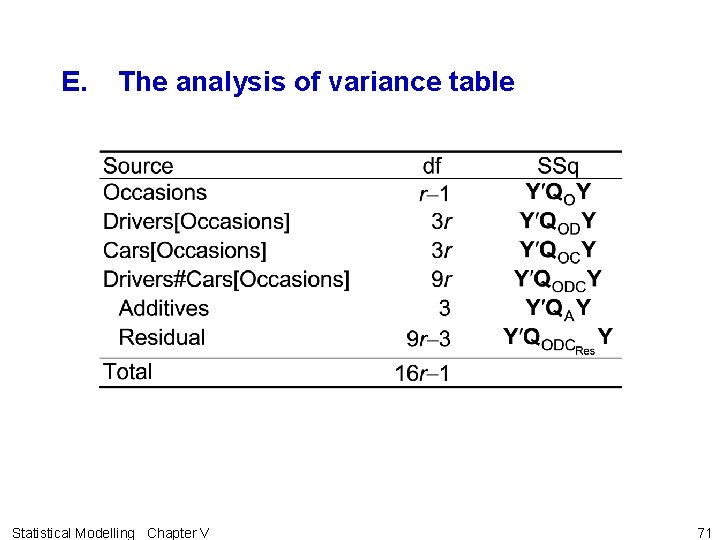
E. The analysis of variance table Statistical Modelling Chapter V 71

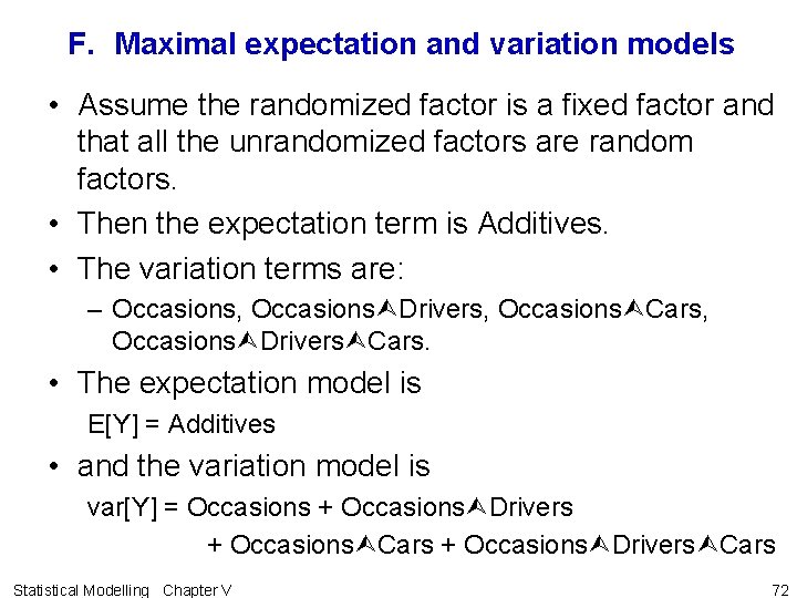
F. Maximal expectation and variation models • Assume the randomized factor is a fixed factor and that all the unrandomized factors are random factors. • Then the expectation term is Additives. • The variation terms are: – Occasions, Occasions Drivers, Occasions Cars, Occasions Drivers Cars. • The expectation model is E[Y] = Additives • and the variation model is var[Y] = Occasions + Occasions Drivers + Occasions Cars + Occasions Drivers Cars Statistical Modelling Chapter V 72

G. The expected mean squares • The Hasse diagram, with contributions to E[MSq]s, for the unrandomized factors in this study is left as an exercise. • The single randomized factor Additive will contribute q. A(y) to the E[MSq] for its source. ANOVA table with E[MSq] • Hypothesis tests for Drivers[Occasions], Cars[Occasions] and Additives are straightforward • The test for Occasions is more difficult. Statistical Modelling Chapter V 73

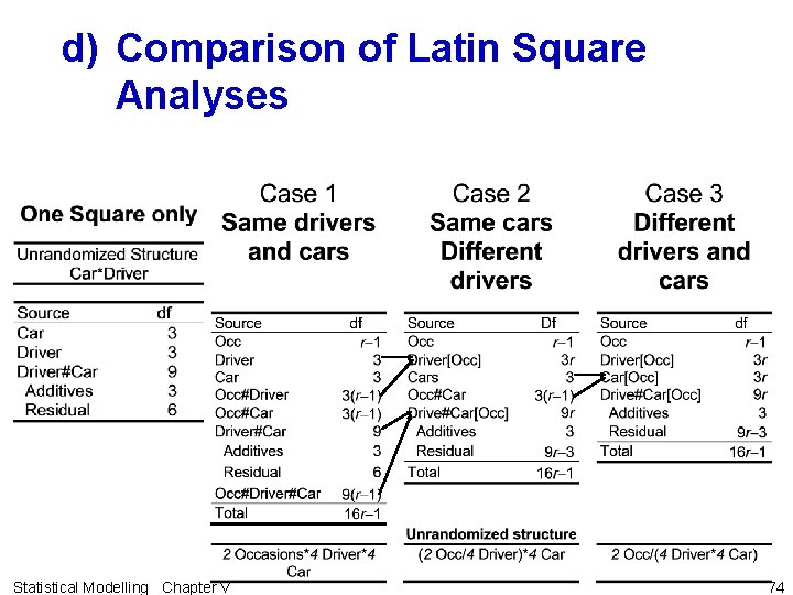
d) Comparison of Latin Square Analyses Statistical Modelling Chapter V 74

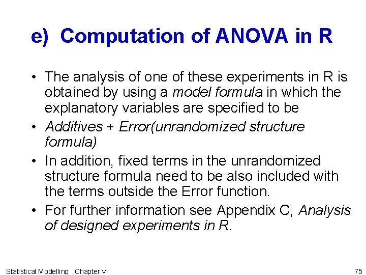
e) Computation of ANOVA in R • The analysis of one of these experiments in R is obtained by using a model formula in which the explanatory variables are specified to be • Additives + Error(unrandomized structure formula) • In addition, fixed terms in the unrandomized structure formula need to be also included with the terms outside the Error function. • For further information see Appendix C, Analysis of designed experiments in R. Statistical Modelling Chapter V 75

V. I Exercises • Ex. V-1 asks for a randomized layout for a Latin square • Ex. V-2 looks at random versus fixed effects • Ex. V-3 asks for the complete analysis of an LSD with a qualitative treatment factor • Ex. V-4 investigates the design and analysis of Sets of Latin squares Statistical Modelling Chapter V 76