v Estimator Definitions a formula or process for

v Estimator Definitions a formula or process for using sample data to estimate a population parameter v Estimate a specific value or range of values used to approximate some population parameter v Point Estimate a single value (or point) used to approximate a population parameter 1

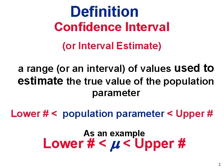
Definition Confidence Interval (or Interval Estimate) a range (or an interval) of values used to estimate the true value of the population parameter Lower # < population parameter < Upper # As an example Lower # < < Upper # 2

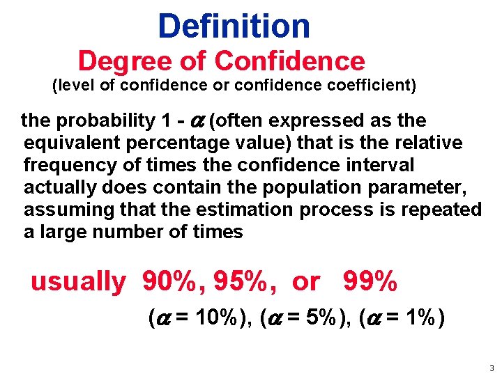
Definition Degree of Confidence (level of confidence or confidence coefficient) the probability 1 - (often expressed as the equivalent percentage value) that is the relative frequency of times the confidence interval actually does contain the population parameter, assuming that the estimation process is repeated a large number of times usually 90%, 95%, or 99% ( = 10%), ( = 5%), ( = 1%) 3

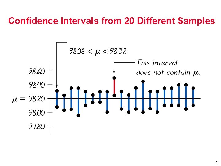
Confidence Intervals from 20 Different Samples 4

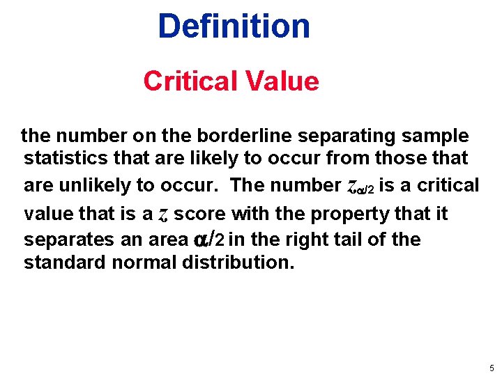
Definition Critical Value the number on the borderline separating sample statistics that are likely to occur from those that are unlikely to occur. The number z /2 is a critical value that is a z score with the property that it separates an area /2 in the right tail of the standard normal distribution. 5

Assumptions v n > 30 The sample must have more than 30 values. v Simple Random Sample All samples of the same size have an equal chance of being selected. Data collected carelessly can be absolutely worthless, even if the sample is quite large. 6

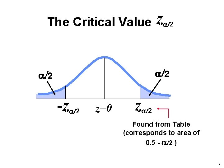
The Critical Value z 2 2 2 -z 2 z=0 z 2 Found from Table (corresponds to area of 0. 5 - 2 ) 7

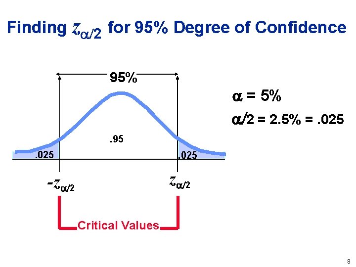
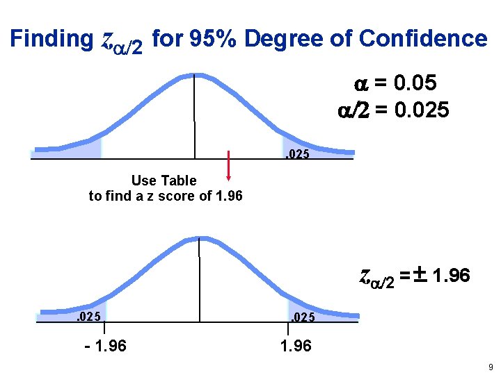
Finding z 2 for 95% Degree of Confidence 95% = 5% 2 = 2. 5% =. 025. 95. 025 z 2 -z 2 Critical Values 8

Finding z 2 for 95% Degree of Confidence = 0. 05 = 0. 025 Use Table to find a z score of 1. 96 z 2 = 1. 96. 025 - 1. 96 . 025 1. 96 9

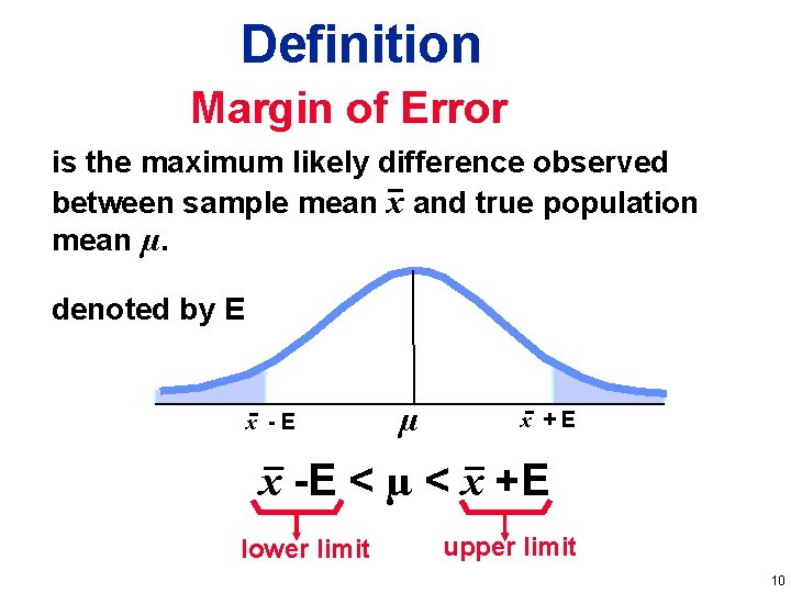
Definition Margin of Error is the maximum likely difference observed between sample mean x and true population mean µ. denoted by E x -E µ x +E x -E < µ < x +E lower limit upper limit 10

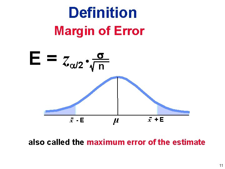
Definition Margin of Error E = z /2 • x -E n µ x +E also called the maximum error of the estimate 11

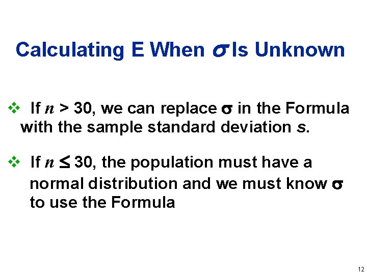
Calculating E When Is Unknown v If n > 30, we can replace in the Formula with the sample standard deviation s. v If n 30, the population must have a normal distribution and we must know to use the Formula 12

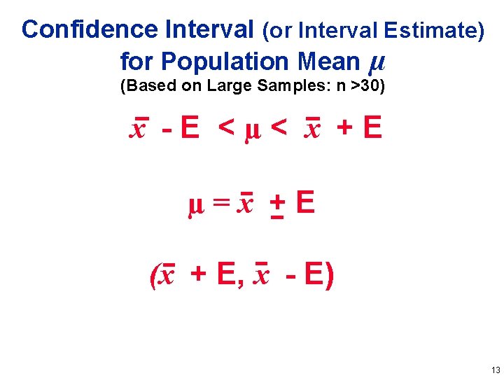
Confidence Interval (or Interval Estimate) for Population Mean µ (Based on Large Samples: n >30) x -E <µ< x +E µ=x +E (x + E, x - E) 13

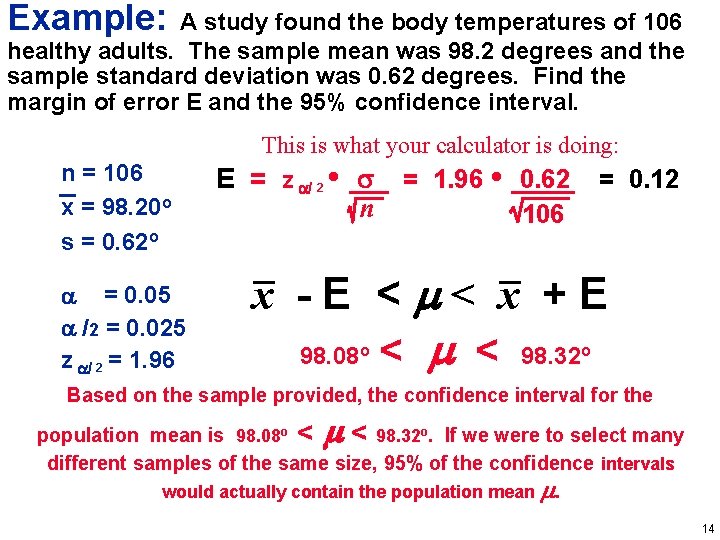
Example: A study found the body temperatures of 106 healthy adults. The sample mean was 98. 2 degrees and the sample standard deviation was 0. 62 degrees. Find the margin of error E and the 95% confidence interval. n = 106 x = 98. 20 o s = 0. 62 o = 0. 05 /2 = 0. 025 z / 2 = 1. 96 This is what your calculator is doing: E = z / 2 • = 1. 96 • 0. 62 = 0. 12 n 106 x -E < < x +E 98. 08 o < < 98. 32 o Based on the sample provided, the confidence interval for the population mean is 98. 08 o < < 98. 32 o. If we were to select many different samples of the same size, 95% of the confidence intervals would actually contain the population mean . 14

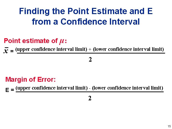
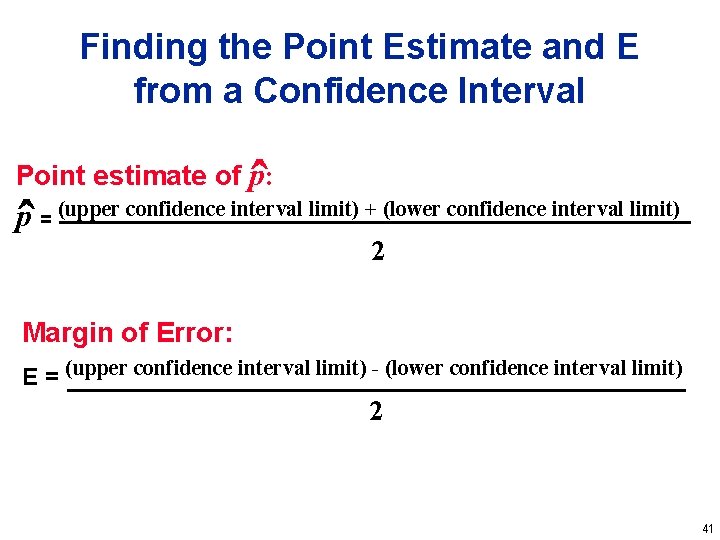
Finding the Point Estimate and E from a Confidence Interval Point estimate of µ: x = (upper confidence interval limit) + (lower confidence interval limit) 2 Margin of Error: E = (upper confidence interval limit) - (lower confidence interval limit) 2 15

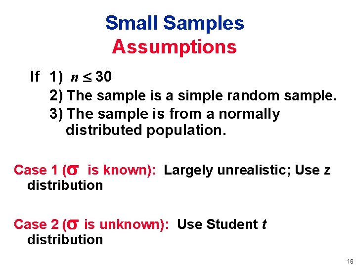
Small Samples Assumptions If 1) n 30 2) The sample is a simple random sample. 3) The sample is from a normally distributed population. Case 1 ( is known): Largely unrealistic; Use z distribution Case 2 ( is unknown): Use Student t distribution 16

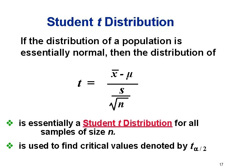
Student t Distribution If the distribution of a population is essentially normal, then the distribution of t = x-µ s n v is essentially a Student t Distribution for all samples of size n. v is used to find critical values denoted by t / 2 17

Table v Formulas and Tables Card v Front cover v Appendix 18

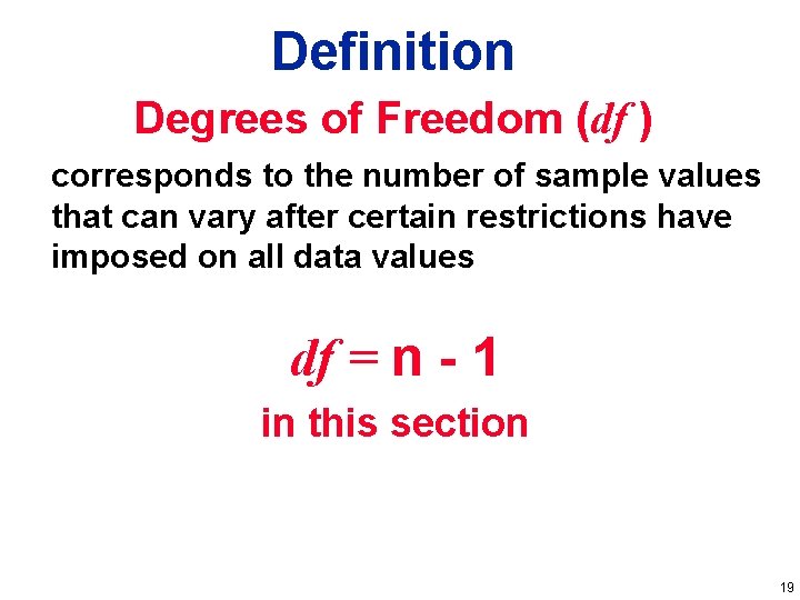
Definition Degrees of Freedom (df ) corresponds to the number of sample values that can vary after certain restrictions have imposed on all data values df = n - 1 in this section 19

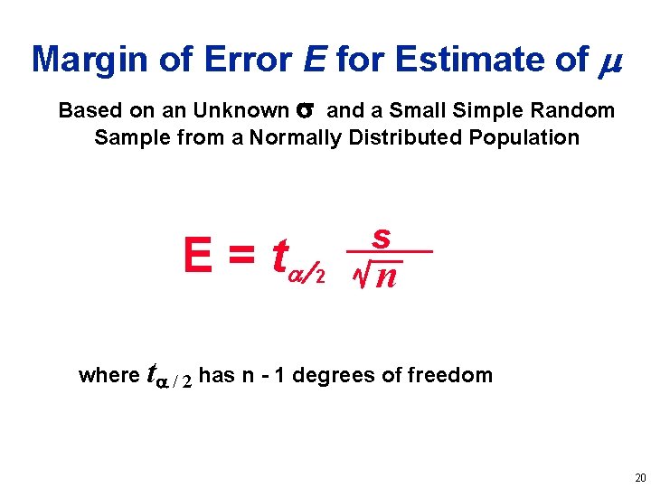
Margin of Error E for Estimate of Based on an Unknown and a Small Simple Random Sample from a Normally Distributed Population E = t s 2 n where t / 2 has n - 1 degrees of freedom 20

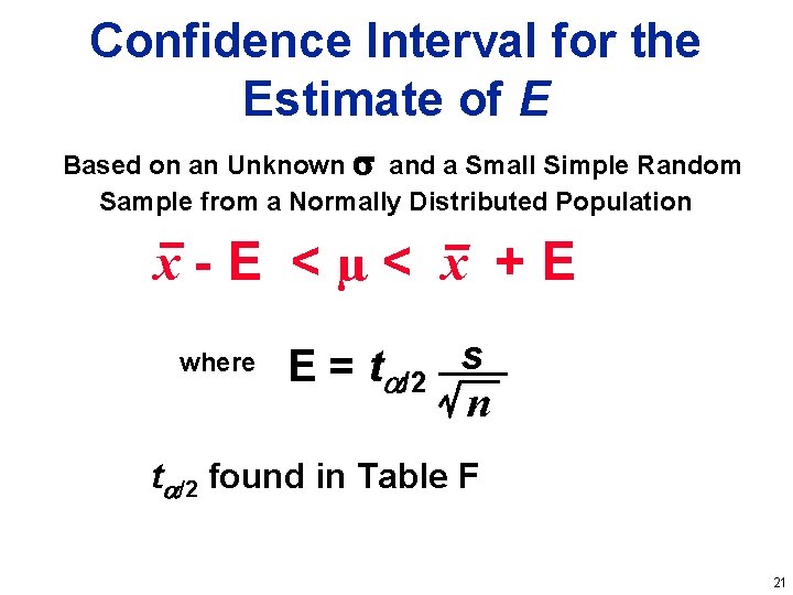
Confidence Interval for the Estimate of E Based on an Unknown and a Small Simple Random Sample from a Normally Distributed Population x-E <µ< x +E where E = t /2 s n t /2 found in Table F 21

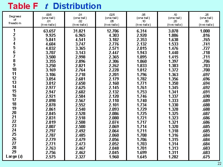
Table F t Distribution Degrees of freedom 1 2 3 4 5 6 7 8 9 10 11 12 13 14 15 16 17 18 19 20 21 22 23 24 25 26 27 28 29 Large (z) . 005 (one tail). 01 (two tails) 63. 657 9. 925 5. 841 4. 604 4. 032 3. 707 3. 500 3. 355 3. 250 3. 169 3. 106 3. 054 3. 012 2. 977 2. 947 2. 921 2. 898 2. 878 2. 861 2. 845 2. 831 2. 819 2. 807 2. 797 2. 787 2. 779 2. 771 2. 763 2. 756 2. 575 . 01 (one tail). 02 (two tails) 31. 821 6. 965 4. 541 3. 747 3. 365 3. 143 2. 998 2. 896 2. 821 2. 764 2. 718 2. 681 2. 650 2. 625 2. 602 2. 584 2. 567 2. 552 2. 540 2. 528 2. 518 2. 500 2. 492 2. 485 2. 479 2. 473 2. 467 2. 462 2. 327 . 025 (one tail). 05 (two tails) 12. 706 4. 303 3. 182 2. 776 2. 571 2. 447 2. 365 2. 306 2. 262 2. 228 2. 201 2. 179 2. 160 2. 145 2. 132 2. 120 2. 110 2. 101 2. 093 2. 086 2. 080 2. 074 2. 069 2. 064 2. 060 2. 056 2. 052 2. 048 2. 045 1. 960 . 05 (one tail). 10 (two tails) . 10 (one tail). 20 (two tails) . 25 (one tail). 50 (two tails) 6. 314 2. 920 2. 353 2. 132 2. 015 1. 943 1. 895 1. 860 1. 833 1. 812 1. 796 1. 782 1. 771 1. 761 1. 753 1. 746 1. 740 1. 734 1. 729 1. 725 1. 721 1. 717 1. 714 1. 711 1. 708 1. 706 1. 703 1. 701 1. 699 1. 645 3. 078 1. 886 1. 638 1. 533 1. 476 1. 440 1. 415 1. 397 1. 383 1. 372 1. 363 1. 356 1. 350 1. 345 1. 341 1. 337 1. 333 1. 330 1. 328 1. 325 1. 323 1. 321 1. 320 1. 318 1. 316 1. 315 1. 314 1. 313 1. 311 1. 282 1. 000. 816. 765. 741. 727. 718. 711. 706. 703. 700. 697. 696. 694. 692. 691. 690. 689. 688. 687. 686. 685. 684. 683. 675 22

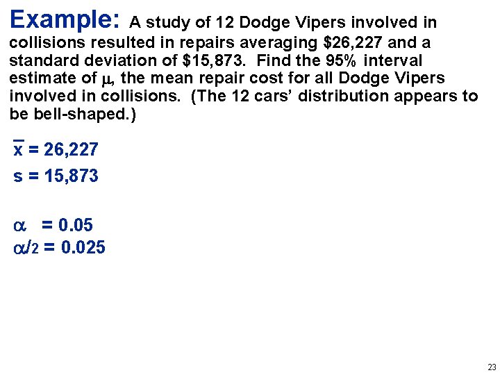
Example: A study of 12 Dodge Vipers involved in collisions resulted in repairs averaging $26, 227 and a standard deviation of $15, 873. Find the 95% interval estimate of , the mean repair cost for all Dodge Vipers involved in collisions. (The 12 cars’ distribution appears to be bell-shaped. ) x = 26, 227 s = 15, 873 = 0. 05 /2 = 0. 025 23

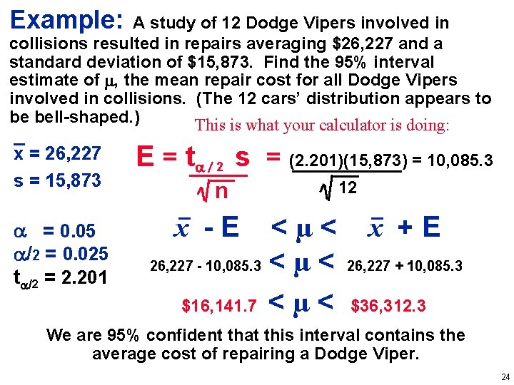
Example: A study of 12 Dodge Vipers involved in collisions resulted in repairs averaging $26, 227 and a standard deviation of $15, 873. Find the 95% interval estimate of , the mean repair cost for all Dodge Vipers involved in collisions. (The 12 cars’ distribution appears to be bell-shaped. ) This is what your calculator is doing: x = 26, 227 s = 15, 873 = 0. 05 /2 = 0. 025 t /2 = 2. 201 E = t 2 s = (2. 201)(15, 873) = 10, 085. 3 n x -E <µ< 26, 227 - 10, 085. 3 < µ < $16, 141. 7 < µ < 12 x +E 26, 227 + 10, 085. 3 $36, 312. 3 We are 95% confident that this interval contains the average cost of repairing a Dodge Viper. 24

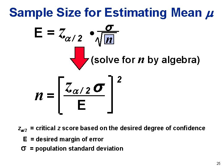
Sample Size for Estimating Mean E = z / 2 • n (solve for n by algebra) n= z / 2 2 E z /2 = critical z score based on the desired degree of confidence E = desired margin of error = population standard deviation 25

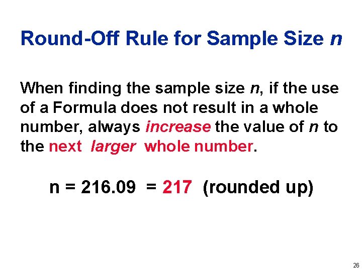
Round-Off Rule for Sample Size n When finding the sample size n, if the use of a Formula does not result in a whole number, always increase the value of n to the next larger whole number. n = 216. 09 = 217 (rounded up) 26

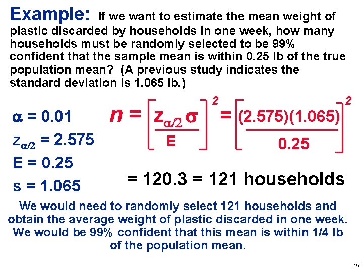
Example: If we want to estimate the mean weight of plastic discarded by households in one week, how many households must be randomly selected to be 99% confident that the sample mean is within 0. 25 lb of the true population mean? (A previous study indicates the standard deviation is 1. 065 lb. ) 2 2 = 0. 01 z = 2. 575 E = 0. 25 s = 1. 065 n = z E = (2. 575)(1. 065) 0. 25 = 120. 3 = 121 households We would need to randomly select 121 households and obtain the average weight of plastic discarded in one week. We would be 99% confident that this mean is within 1/4 lb of the population mean. 27

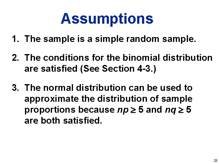
Assumptions 1. The sample is a simple random sample. 2. The conditions for the binomial distribution are satisfied (See Section 4 -3. ) 3. The normal distribution can be used to approximate the distribution of sample proportions because np 5 and nq 5 are both satisfied. 28

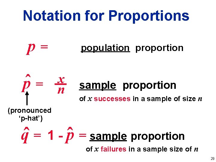
Notation for Proportions p= ˆp = nx population proportion sample proportion of x successes in a sample of size n (pronounced ‘p-hat’) qˆ = 1 - pˆ = sample proportion of x failures in a sample size of n 29

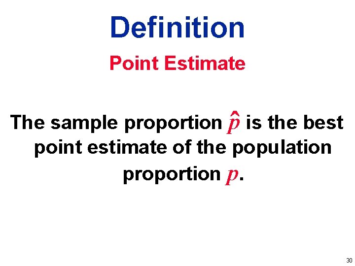
Definition Point Estimate The sample proportion p ˆ is the best point estimate of the population proportion p. 30

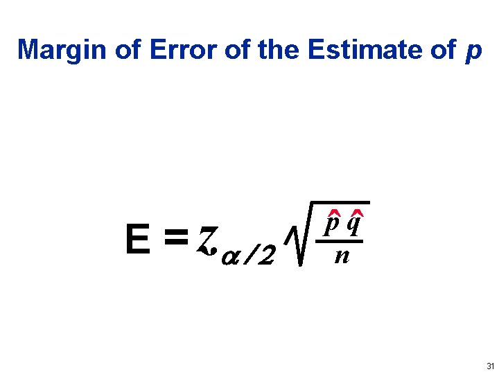
Margin of Error of the Estimate of p E = z pˆ qˆ n 31

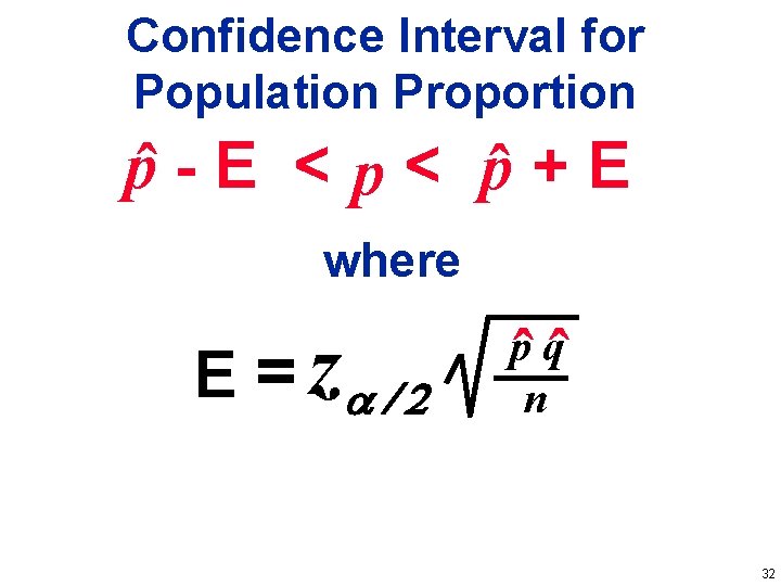
Confidence Interval for Population Proportion pˆ - E < pˆ + E where E = z pˆ qˆ n 32

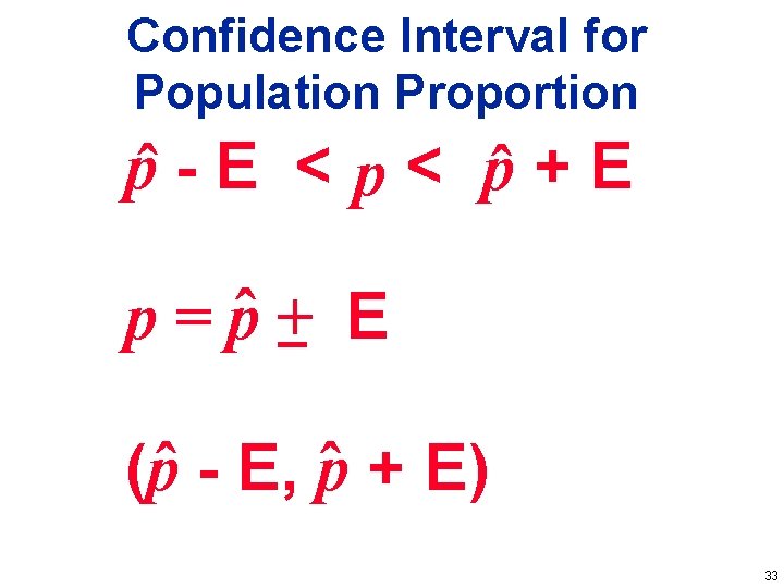
Confidence Interval for Population Proportion pˆ - E < pˆ + E p = pˆ + E (pˆ - E, pˆ + E) 33

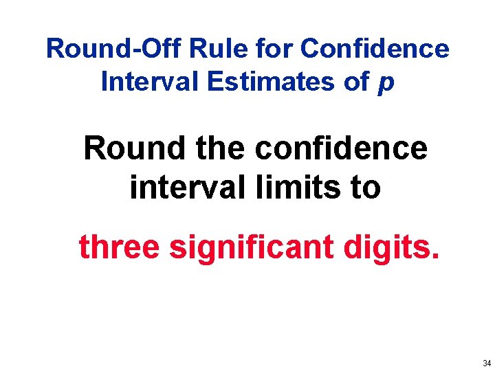
Round-Off Rule for Confidence Interval Estimates of p Round the confidence interval limits to three significant digits. 34

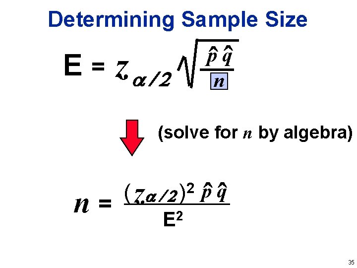
Determining Sample Size E = z pˆ qˆ n (solve for n by algebra) n= 2 pq ( z ) ˆˆ E 2 35

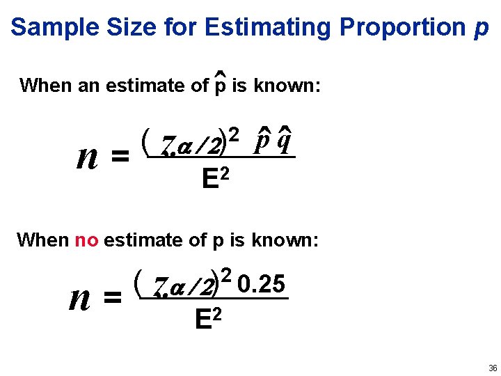
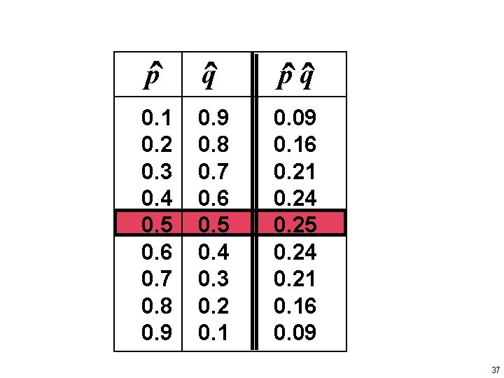
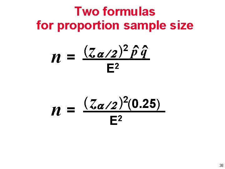
Sample Size for Estimating Proportion p ˆ When an estimate of p is known: n pˆ qˆ ( z = 2 2 ) E When no estimate of p is known: n 2 0. 25 ( z ) = 2 E 36

pˆ qˆ 0. 1 0. 2 0. 3 0. 4 0. 5 0. 6 0. 7 0. 8 0. 9 0. 8 0. 7 0. 6 0. 5 0. 4 0. 3 0. 2 0. 1 0. 09 0. 16 0. 21 0. 24 0. 25 0. 24 0. 21 0. 16 0. 09 37

Two formulas for proportion sample size n= n= ( z )2 pˆ qˆ E 2 ( z (0. 25) 2 ) E 2 38

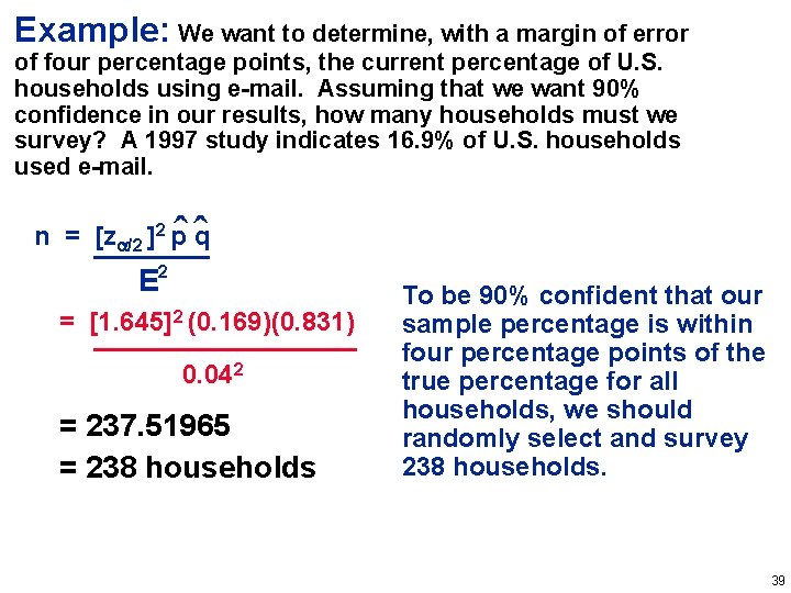
Example: We want to determine, with a margin of error of four percentage points, the current percentage of U. S. households using e-mail. Assuming that we want 90% confidence in our results, how many households must we survey? A 1997 study indicates 16. 9% of U. S. households used e-mail. ˆˆ n = [z /2 ]2 p q E 2 = [1. 645]2 (0. 169)(0. 831) 0. 042 = 237. 51965 = 238 households To be 90% confident that our sample percentage is within four percentage points of the true percentage for all households, we should randomly select and survey 238 households. 39

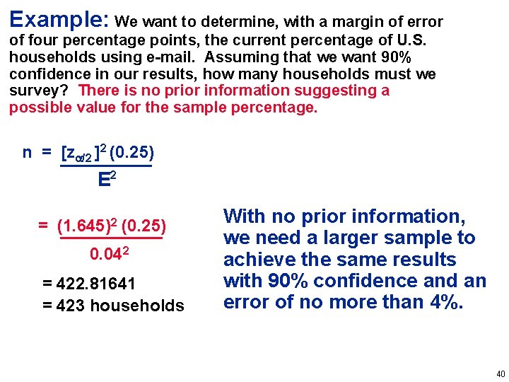
Example: We want to determine, with a margin of error of four percentage points, the current percentage of U. S. households using e-mail. Assuming that we want 90% confidence in our results, how many households must we survey? There is no prior information suggesting a possible value for the sample percentage. n = [z /2 ]2 (0. 25) E 2 = (1. 645)2 (0. 25) 0. 042 = 422. 81641 = 423 households With no prior information, we need a larger sample to achieve the same results with 90% confidence and an error of no more than 4%. 40

Finding the Point Estimate and E from a Confidence Interval ˆ (upper confidence interval limit) + (lower confidence interval limit) Point estimate of p: ˆ p= 2 Margin of Error: E = (upper confidence interval limit) - (lower confidence interval limit) 2 41

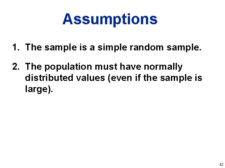
Assumptions 1. The sample is a simple random sample. 2. The population must have normally distributed values (even if the sample is large). 42

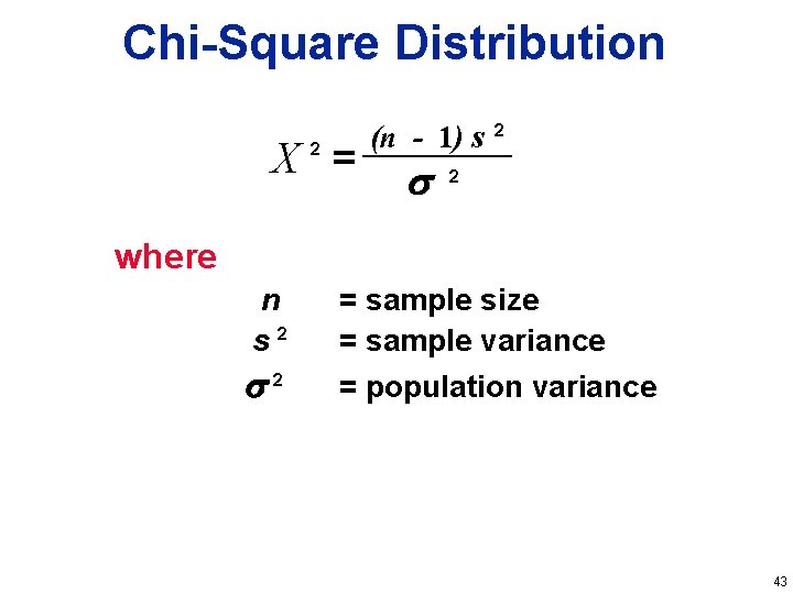
Chi-Square Distribution X = 2 (n - 1) s 2 2 where n s 2 2 = sample size = sample variance = population variance 43

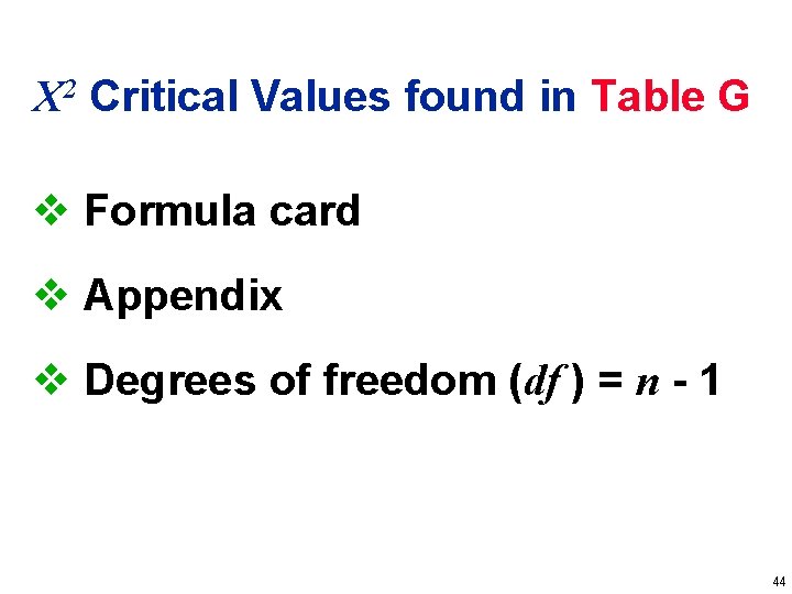
X 2 Critical Values found in Table G v Formula card v Appendix v Degrees of freedom (df ) = n - 1 44

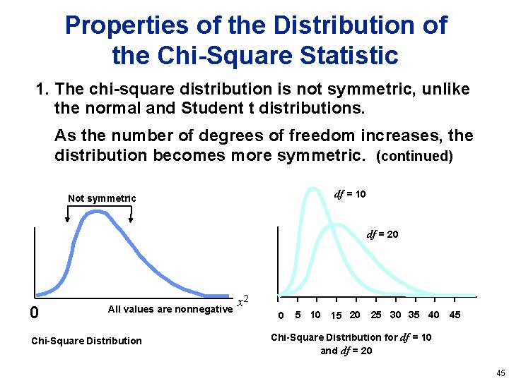
Properties of the Distribution of the Chi-Square Statistic 1. The chi-square distribution is not symmetric, unlike the normal and Student t distributions. As the number of degrees of freedom increases, the distribution becomes more symmetric. (continued) df = 10 Not symmetric df = 20 0 All values are nonnegative Chi-Square Distribution x 2 0 5 10 15 20 25 30 35 40 45 Chi-Square Distribution for df = 10 and df = 20 45

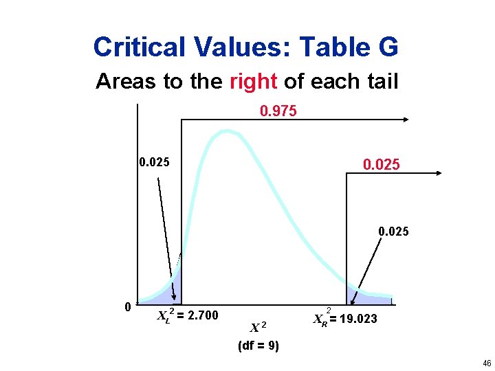
Critical Values: Table G Areas to the right of each tail 0. 975 0. 025 0 XL 2 = 2. 700 2 X 2 (df = 9) XR = 19. 023 46

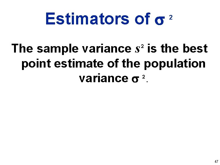
Estimators of 2 The sample variance s is the best point estimate of the population variance . 2 2 47

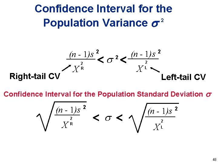
Confidence Interval for the 2 Population Variance (n - 1)s 2 X Right-tail CV 2 R 2 (n - 1)s 2 X 2 L Left-tail CV Confidence Interval for the Population Standard Deviation (n - 1)s 2 X 2 R (n - 1)s 2 2 XL 48

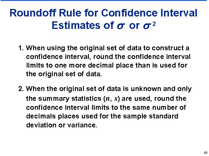
Roundoff Rule for Confidence Interval Estimates of or 2 1. When using the original set of data to construct a confidence interval, round the confidence interval limits to one more decimal place than is used for the original set of data. 2. When the original set of data is unknown and only the summary statistics (n, s) are used, round the confidence interval limits to the same number of decimals places used for the sample standard deviation or variance. 49