V Dynamics of ConsumerResource Interactions A Predators can

V. Dynamics of Consumer-Resource Interactions A. Predators can limit the growth of prey populations B. Oscillations are a Common Pattern C. Models 1. Host-Pathogen Models

V. Dynamics of Consumer-Resource Interactions A. Predators can limit the growth of prey populations B. Oscillations are a Common Pattern C. Models 1. Host-Pathogen Models Dependent on: a. the rate of transmission (b) (“infectability”) b. the rate of recovery (g) (inversely related to the period during which the host is contagious) c. the number of susceptible (S), infectious, and recovered hosts

V. Dynamics of Consumer-Resource Interactions A. Predators can limit the growth of prey populations B. Oscillations are a Common Pattern C. Models 1. Host-Pathogen Models Dependent on: a. the rate of transmission (b) b. the rate of recovery (g) (inversely related to the period during which the host is contagious) c. the number of susceptible (S), infectious, and recovered hosts The reproductive ratio of the pathogen =(b/g)S so a pathogen population will grow (R > 1, epidemic) if : the rate of transmission is high (infectious) recovery is slow (creating a long period of contagion) susceptible individuals are common. In this case, each infected individual infects more than one new host and the disease spreads.

V. Dynamics of Consumer-Resource Interactions A. Predators can limit the growth of prey populations B. Oscillations are a Common Pattern C. Models 1. Host-Pathogen Models As a disease proceeds and the number of susceptible individuals declines, R < 1 and the epidemic declines. In the simplest version of this model (single generation), oscillations don’t occur because there is no production of new susceptible people and immunity after recovery is permanent. However, if you add the production of susceptible newborns or susceptible immigrants, or allow for vertical transmission from parent to offspring, or add a latency period, or allow for reinfection (and not lifetime immunity), oscillations and cyclic epidemic occur because the number of susceptible people can increase… driving R > 1.

so a pathogen population will grow (R > 1, epidemic) if : the rate of transmission is high recovery is slow (creating a long period of contagion) or susceptible individuals are common. In this case, each infected individual infects more than one new host and the disease spreads. Cold and Flu: Transmission rate “low” - 34% Recovery slow, favoring spread (Viral integrity is greatest under low humidity, and particles remain small (don’t take on water and fall out of the air column). Cool temps reduce ciliary beating in nasal and respiratory mucosa, favoring viral reproduction. Both cause higher transmission rates in winter. Lowen, et al. 2007. http: //www. plospathogens. org/article/info%3 Adoi%2 F 10. 1371%2 Fjournal. ppat. 0030151

so a pathogen population will grow (R > 1, epidemic) if : the rate of transmission is high recovery is slow (creating a long period of contagion) or susceptible individuals are common. In this case, each infected individual infects more than one new host and the disease spreads. Ebola: Transmission rate “high” ~75% 99% fatality rate – short contagious period Deadly pathogens need a high transmission rate to persist, or a very dense population (S).

so a pathogen population will grow (R > 1, epidemic) if : the rate of transmission is high recovery is slow (creating a long period of contagion) or susceptible individuals are common. In this case, each infected individual infects more than one new host and the disease spreads. 1918 Flu Epidemic (H 1 N 1): Killed 50 -100 million people; 3 -5% of the global population Transmission rate was high because of high density of susceptible hosts (military), and movement of carriers across Europe (military and migrating refugees). High density selected for more aggressive and lethal form

Reduce Transmission Rate: - stay clean - stay home Reduce Contagious Period: - stay healthy Reduce # of Susceptible Hosts: - get vaccinated

C. Models 1. Host-Pathogen Model 2. Lotka-Volterra Models Goal - create a model system in which there are oscillations of predator and prey populations that are out-of-phase with one another. Basic Equations: a. Prey (V = ‘victim’) Equation: d. V/dt = r. V - c. VP where r. V defines the maximal, exponential rate c = predator foraging efficiency: % eaten P = number of predators V= number of prey, so PV = number of encounters and c. PV = number of prey killed (consumed) So, the formula describes the maximal growth rate, minus the number of prey individuals lost by predation.

The Prey Isocline d. V/dt = 0 when r. V = c. PV; when P = r/c. Curious dynamic. There is a particular number of predators that can limit prey growth; below this number of predators, REGARDLESS OF THE NUMBER OF PREY, prey increase. Greater than this number of predators, REGARDLESS OF THE NUMBER OF PREY, and the prey declines. Prey's rate of growth is independent of its own density (rather unrealistic). r/c V

C. Models 2. Lotka-Volterra Models b. Predator The Equation: d. P/dt = a(c. PV) - d. P where c. PV equals the number of prey consumed, and a = the rate at which food energy is converted to offspring. So, a(c. VP) = number of predator offspring produced. d = mortality rate, and P = # of predators, so d. P = number of predators dying. So, the equation boils down to the birth rate (determined by energy "in" and conversion rate to offspring) minus the death rate.

The Predator's Isocline d. P/dt = 0 when d. P = a(c. PV); or when V = d/ac Again, Predator's growth is independent of its own density. There is a critical number of prey which can support a predator population of any size; below this number, the predator population declines - above this number and the population can increase. V d/ac

Basic Equations: 1. Prey 2. Predator 3. Dynamics d/ac 1. 4. 1. 2. 3. 4. V r/c 2. 3. OSCILLATIONS!!! (V) 1.

Curiously, the model predicts that an increase in the growth rate of prey (r to r’) (favorable change in the environment? ) should NOT change equilibrial PREY density (d/ac), but instead should cause PREDATOR population to grow to higher equilibrium (r’/c). Experimental Support: - Increase sugar to E. coli bacteria, and their population did not increase much as the predators (T 4 phage) increased.

- Criticisms of the L-V model: 1. No time lags – instantaneous conversion of food to predator offspring 2. No density dependence in prey, even at low predator densities when prey populations should be large. 3. Constant predation rate (functional response)

V. Dynamics of Consumer-Resource Interactions A. Predators can limit the growth of prey populations B. Oscillations are a Common Pattern C. Models D. Lab Experiments 1. Gause P. caudatum (prey) and Didinium nasutum (predator)

P. caudatum (prey) and Didinium nasutum (predator) In initial experiments, Paramecium populations would increase, followed by a pulse of Didinium, and then they would crash.

P. caudatum (prey) and Didinium nasutum (predator) In initial experiments, Paramecium populations would increase, followed by a pulse of Didinium, and then they would crash. He added glass wool to the bottom, creating a REFUGE that the predator did not enter.

He induced oscillations by adding Paramecium as 'immigrants'

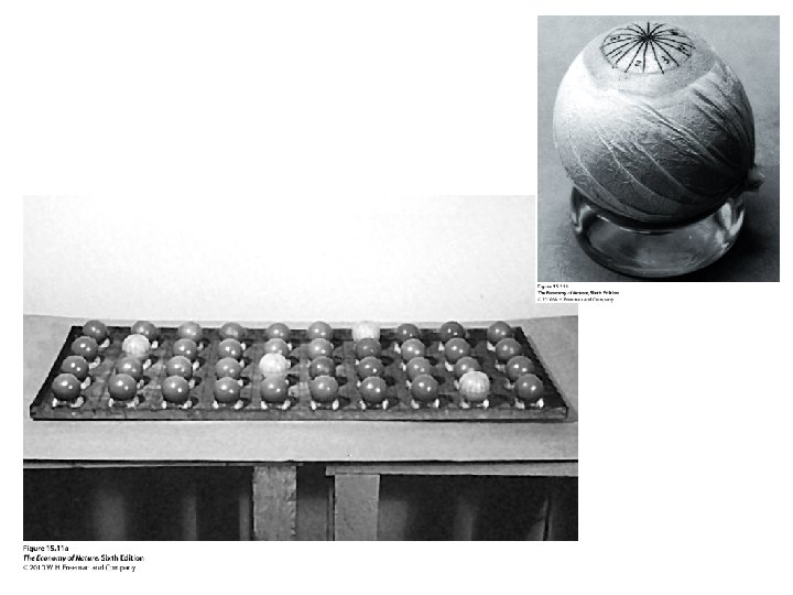
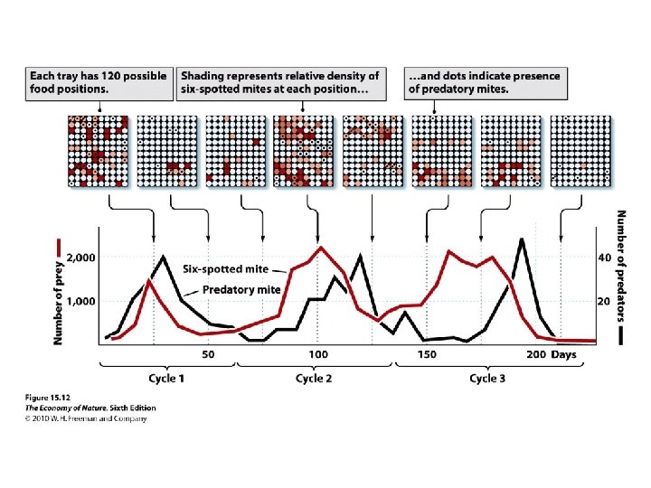
D. Laboratory Experiments 1. Gause 2. Huffaker six-spotted mite (Eotetranychus sexmaculatus) was prey - SSM Predatory mite (Typhlodromus occidentalis) was predator - PM

D. Complexities and Applications 1. Achieving Stable Dynamics - inefficient predators: - both populations equilibrate at high density - alternate prey: - Pred’s high, prey low (but not extinct if predator switches) - prey refuge: - prey population dependent on size of the refuge - time lags: - reduced lag allows predator population to equilibrate with changes in prey, and less likely to go extinct by a crash.

D. Complexities and Applications 2. Multiple States Consider a Type III functional response, where the predation rate is highest at intermediate prey densities, and density dependent birth rate of prey. Birth rate Predation Rate V

D. Complexities and Applications 2. Multiple States Consider a Type III functional response, where the predation rate is highest at intermediate prey densities, and density dependent birth rate of prey. Two stable Equilibria, at high and low prey densities. One unstable equilibrium at intermediate density. Birth rate Predation Rate V