V 4 Matrix algorithms and graph partitioning Community

V 4 Matrix algorithms and graph partitioning - Community detection - Simple modularity maximization - Spectral modularity maximization - Division into more than two groups - Other algorithms for community detection SS 2014 - lecture 4 Mathematics of Biological Networks 1

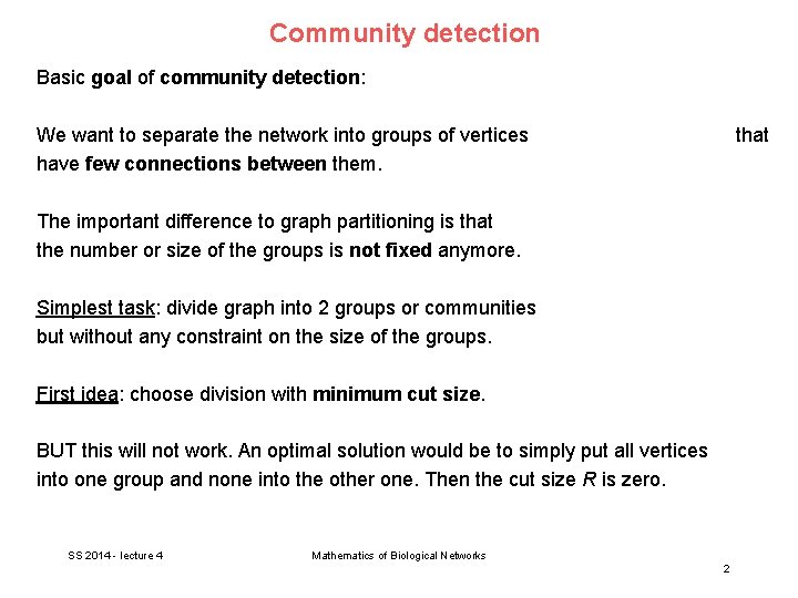
Community detection Basic goal of community detection: We want to separate the network into groups of vertices have few connections between them. that The important difference to graph partitioning is that the number or size of the groups is not fixed anymore. Simplest task: divide graph into 2 groups or communities but without any constraint on the size of the groups. First idea: choose division with minimum cut size. BUT this will not work. An optimal solution would be to simply put all vertices into one group and none into the other one. Then the cut size R is zero. SS 2014 - lecture 4 Mathematics of Biological Networks 2

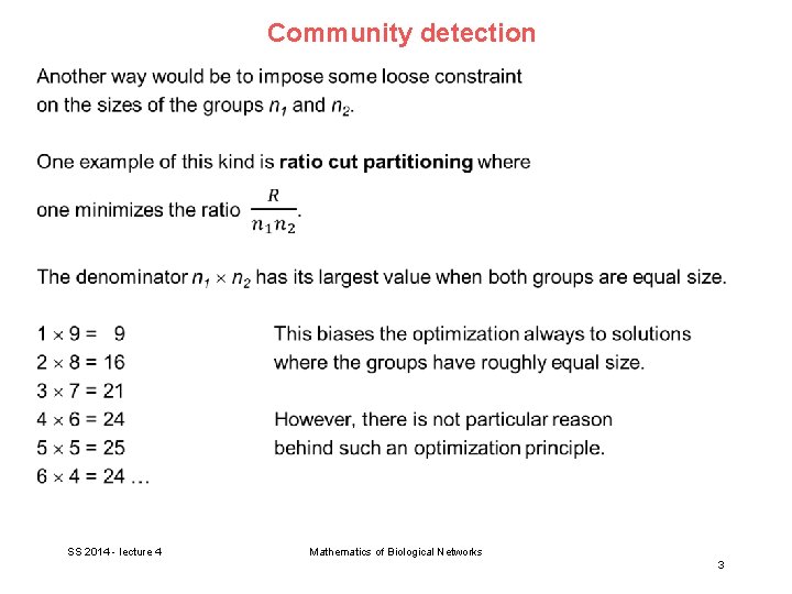
Community detection SS 2014 - lecture 4 Mathematics of Biological Networks 3

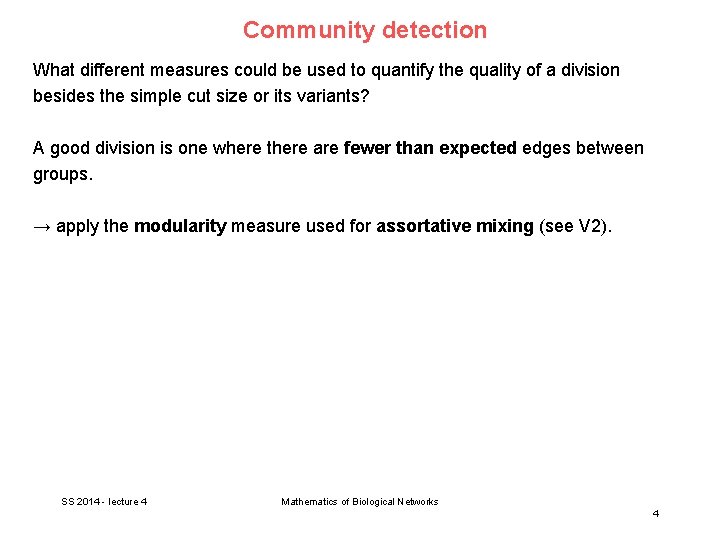
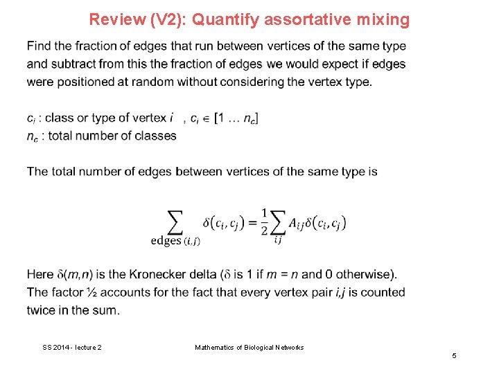
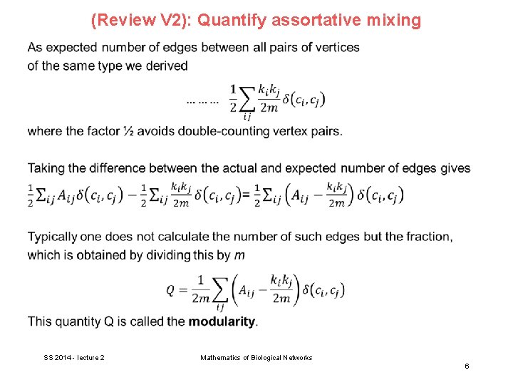
Community detection What different measures could be used to quantify the quality of a division besides the simple cut size or its variants? A good division is one where there are fewer than expected edges between groups. → apply the modularity measure used for assortative mixing (see V 2). SS 2014 - lecture 4 Mathematics of Biological Networks 4

Review (V 2): Quantify assortative mixing SS 2014 - lecture 2 Mathematics of Biological Networks 5

(Review V 2): Quantify assortative mixing SS 2014 - lecture 2 Mathematics of Biological Networks 6

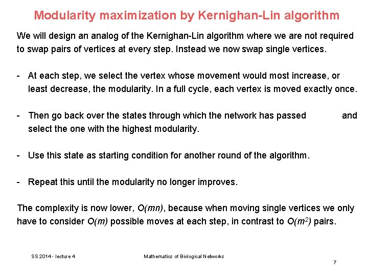
Modularity maximization by Kernighan-Lin algorithm We will design an analog of the Kernighan-Lin algorithm where we are not required to swap pairs of vertices at every step. Instead we now swap single vertices. - At each step, we select the vertex whose movement would most increase, or least decrease, the modularity. In a full cycle, each vertex is moved exactly once. - Then go back over the states through which the network has passed select the one with the highest modularity. and - Use this state as starting condition for another round of the algorithm. - Repeat this until the modularity no longer improves. The complexity is now lower, O(mn), because when moving single vertices we only have to consider O(m) possible moves at each step, in contrast to O(m 2) pairs. SS 2014 - lecture 4 Mathematics of Biological Networks 7

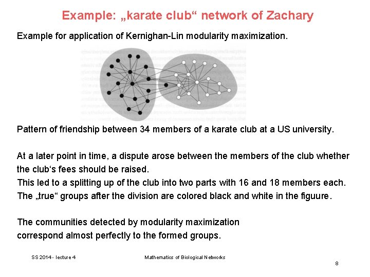
Example: „karate club“ network of Zachary Example for application of Kernighan-Lin modularity maximization. Pattern of friendship between 34 members of a karate club at a US university. At a later point in time, a dispute arose between the members of the club whether the club‘s fees should be raised. This led to a splitting up of the club into two parts with 16 and 18 members each. The „true“ groups after the division are colored black and white in the figuure. The communities detected by modularity maximization correspond almost perfectly to the formed groups. SS 2014 - lecture 4 Mathematics of Biological Networks 8

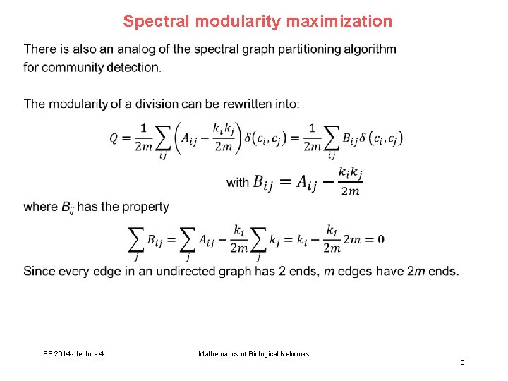
Spectral modularity maximization SS 2014 - lecture 4 Mathematics of Biological Networks 9

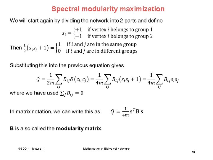
Spectral modularity maximization SS 2014 - lecture 4 Mathematics of Biological Networks 10

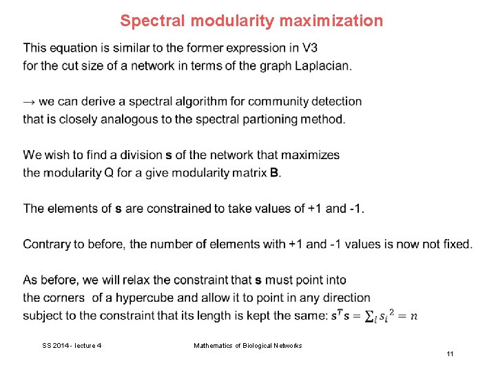
Spectral modularity maximization SS 2014 - lecture 4 Mathematics of Biological Networks 11

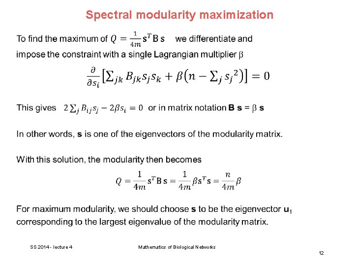
Spectral modularity maximization SS 2014 - lecture 4 Mathematics of Biological Networks 12

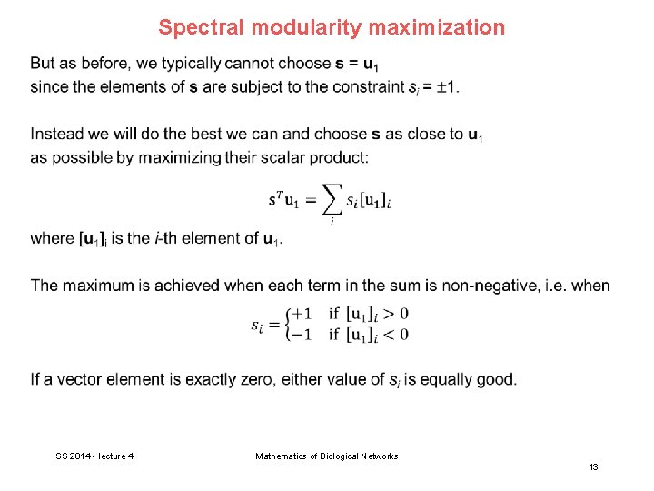
Spectral modularity maximization SS 2014 - lecture 4 Mathematics of Biological Networks 13

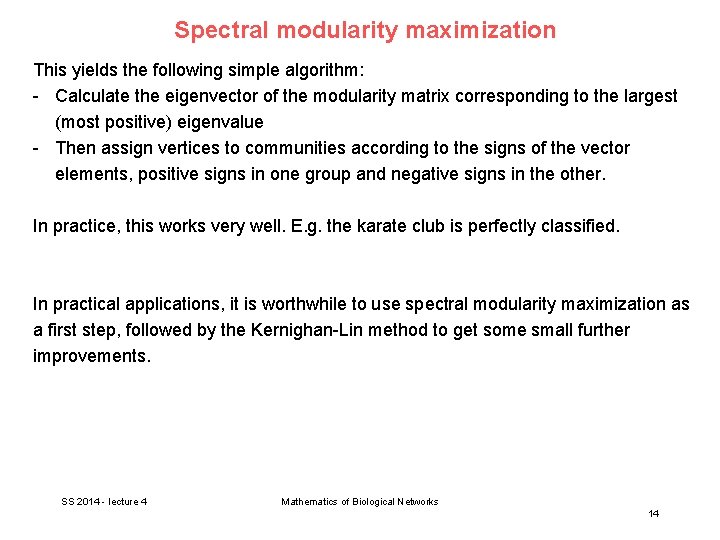
Spectral modularity maximization This yields the following simple algorithm: - Calculate the eigenvector of the modularity matrix corresponding to the largest (most positive) eigenvalue - Then assign vertices to communities according to the signs of the vector elements, positive signs in one group and negative signs in the other. In practice, this works very well. E. g. the karate club is perfectly classified. In practical applications, it is worthwhile to use spectral modularity maximization as a first step, followed by the Kernighan-Lin method to get some small further improvements. SS 2014 - lecture 4 Mathematics of Biological Networks 14

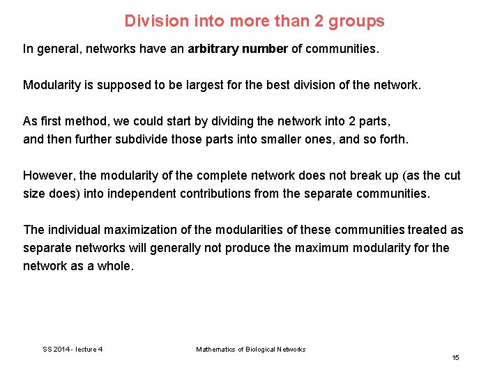
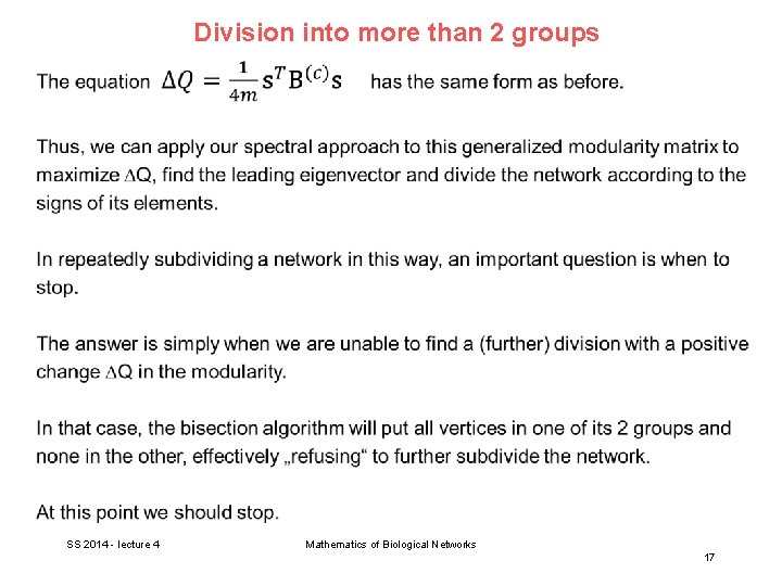
Division into more than 2 groups In general, networks have an arbitrary number of communities. Modularity is supposed to be largest for the best division of the network. As first method, we could start by dividing the network into 2 parts, and then further subdivide those parts into smaller ones, and so forth. However, the modularity of the complete network does not break up (as the cut size does) into independent contributions from the separate communities. The individual maximization of the modularities of these communities treated as separate networks will generally not produce the maximum modularity for the network as a whole. SS 2014 - lecture 4 Mathematics of Biological Networks 15

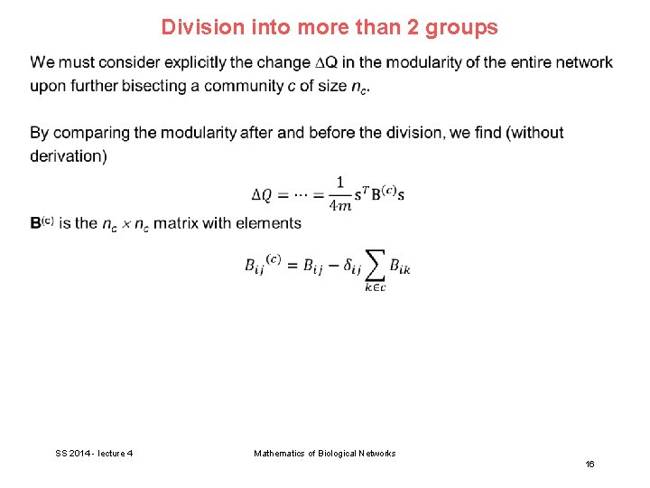
Division into more than 2 groups SS 2014 - lecture 4 Mathematics of Biological Networks 16

Division into more than 2 groups SS 2014 - lecture 4 Mathematics of Biological Networks 17

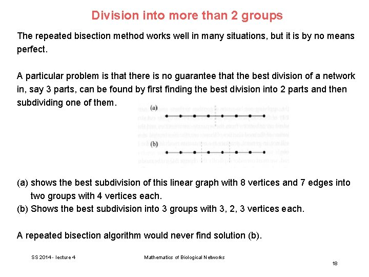
Division into more than 2 groups The repeated bisection method works well in many situations, but it is by no means perfect. A particular problem is that there is no guarantee that the best division of a network in, say 3 parts, can be found by first finding the best division into 2 parts and then subdividing one of them. (a) shows the best subdivision of this linear graph with 8 vertices and 7 edges into two groups with 4 vertices each. (b) Shows the best subdivision into 3 groups with 3, 2, 3 vertices each. A repeated bisection algorithm would never find solution (b). SS 2014 - lecture 4 Mathematics of Biological Networks 18

Other algorithms for community detection An alternative way of finding communities of vertices in a network is to loook for the edges that lie between communities. If we can find and remove these edges, we will be left with isolated communities. One common way to define „betweenness“ is to use betweenness centrality (V 1). SS 2014 - lecture 4 Mathematics of Biological Networks 19

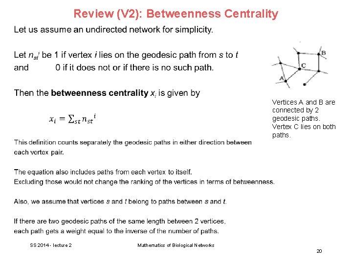
Review (V 2): Betweenness Centrality Vertices A and B are connected by 2 geodesic paths. Vertex C lies on both paths. SS 2014 - lecture 2 Mathematics of Biological Networks 20

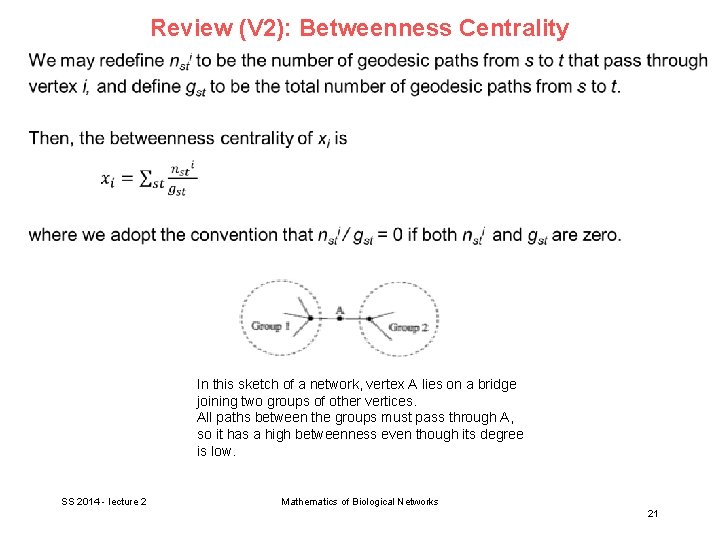
Review (V 2): Betweenness Centrality In this sketch of a network, vertex A lies on a bridge joining two groups of other vertices. All paths between the groups must pass through A, so it has a high betweenness even though its degree is low. SS 2014 - lecture 2 Mathematics of Biological Networks 21

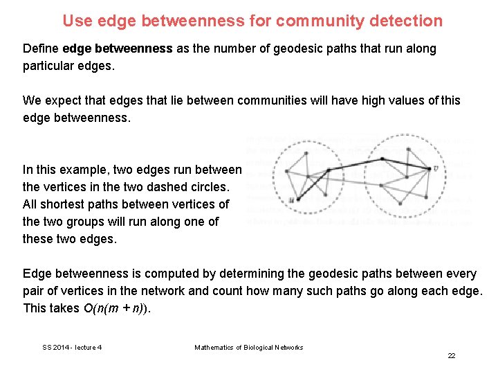
Use edge betweenness for community detection Define edge betweenness as the number of geodesic paths that run along particular edges. We expect that edges that lie between communities will have high values of this edge betweenness. In this example, two edges run between the vertices in the two dashed circles. All shortest paths between vertices of the two groups will run along one of these two edges. Edge betweenness is computed by determining the geodesic paths between every pair of vertices in the network and count how many such paths go along each edge. This takes O(n(m + n)). SS 2014 - lecture 4 Mathematics of Biological Networks 22

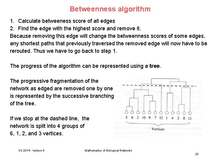
Betweenness algorithm 1. Calculate betweeness score of all edges 2. Find the edge with the highest score and remove it. Because removing this edge will change the betweenness scores of some edges, any shortest paths that previously traversed the removed edge will now have to be rerouted. Thus we have to go back to step 1. The progress of the algorithm can be represented using a tree. The progressive fragmentation of the network as edged are removed one by one is represented by the successive branching of the tree. If we stop at the dashed line, the network is split into 4 groups of 6, 1, 2, and 3 vertices. SS 2014 - lecture 4 Mathematics of Biological Networks 23

Hierarchical clustering Network division by edge betweenness produced a dendrogram that is remiscent of clustering methods. Hierarchical clustering is an entire class of algorithms. It is an agglomerative technique where we start with the individual vertices of a network and join them together to form groups. We need a measure of vertex similarity. For this, we can use the measures introduced in V 1 and V 2, e. g. - cosine similarity, - correlation coefficients between rows of the adjacency matrix, - or the so-called Euclidian distance. Having many choices for similarity measures is both a strength and a weakness of hierarchical clustering methods. It gives the method flexibility, but the results will differ from one another. SS 2014 - lecture 4 Mathematics of Biological Networks 24

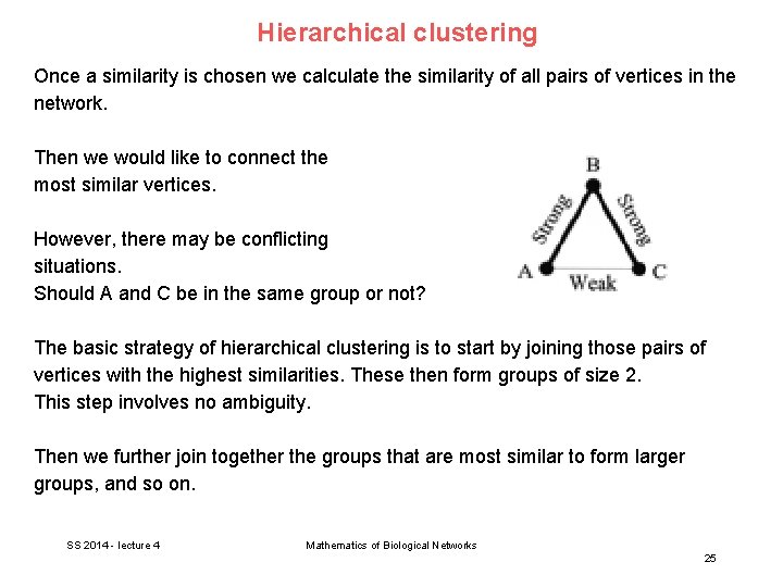
Hierarchical clustering Once a similarity is chosen we calculate the similarity of all pairs of vertices in the network. Then we would like to connect the most similar vertices. However, there may be conflicting situations. Should A and C be in the same group or not? The basic strategy of hierarchical clustering is to start by joining those pairs of vertices with the highest similarities. These then form groups of size 2. This step involves no ambiguity. Then we further join together the groups that are most similar to form larger groups, and so on. SS 2014 - lecture 4 Mathematics of Biological Networks 25

Hierarchical clustering During this process we now require a measure for the similarity of groups. There are 3 common ways of combining vertex similarities to give similarity scores for groups: - single-linkage - complete-linkage - average-linkage clustering. Consider 2 groups of vertices, group 1 and group 2, with n 1 and n 2 vertices, respectively. Then there are n 1 n 2 pairs of vertices such that one vertex is in group 1 and the other in group 2. In the single-linkage clustering method, the similarity between the 2 groups is defined as the similarity of the most similar of these n 1 n 2 pairs of vertices. SS 2014 - lecture 4 Mathematics of Biological Networks 26

Hierarchical clustering In the single-linkage clustering method, the similarity between the 2 groups is defined as the similarity of the most similar of these n 1 n 2 pairs of vertices. As the other extreme, complete-linkage clustering defines the similarity between the 2 groups as the similarity of the least similar pair of vertices. In between these two extremes is the average-linkage clustering where the similarity of two groups is defined to be the mean similarity of all pairs of vertices. SS 2014 - lecture 4 Mathematics of Biological Networks 27

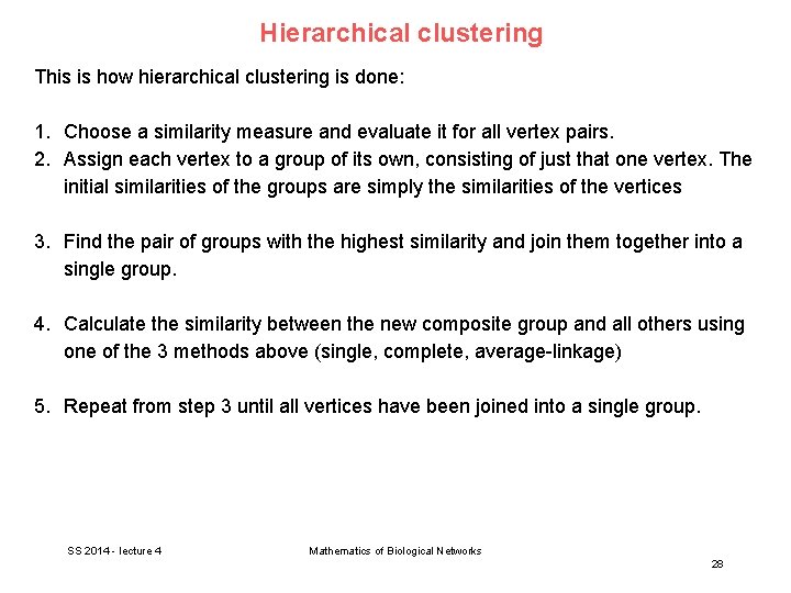
Hierarchical clustering This is how hierarchical clustering is done: 1. Choose a similarity measure and evaluate it for all vertex pairs. 2. Assign each vertex to a group of its own, consisting of just that one vertex. The initial similarities of the groups are simply the similarities of the vertices 3. Find the pair of groups with the highest similarity and join them together into a single group. 4. Calculate the similarity between the new composite group and all others using one of the 3 methods above (single, complete, average-linkage) 5. Repeat from step 3 until all vertices have been joined into a single group. SS 2014 - lecture 4 Mathematics of Biological Networks 28

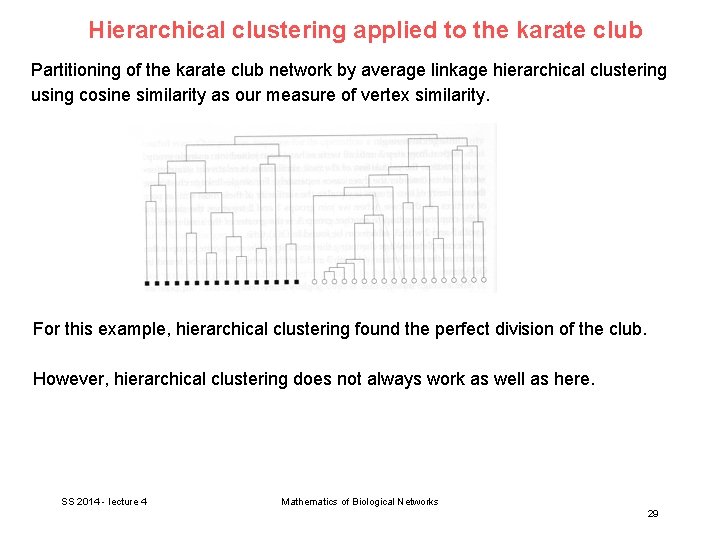
Hierarchical clustering applied to the karate club Partitioning of the karate club network by average linkage hierarchical clustering using cosine similarity as our measure of vertex similarity. For this example, hierarchical clustering found the perfect division of the club. However, hierarchical clustering does not always work as well as here. SS 2014 - lecture 4 Mathematics of Biological Networks 29

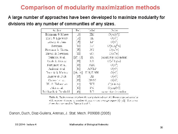
Comparison of modularity maximization methods A large number of approaches have been developed to maximize modularity for divisions into any number of communities of any sizes. Danon, Duch, Diaz-Guilera, Arenas, J. Stat. Mech. P 09008 (2005) SS 2014 - lecture 4 Mathematics of Biological Networks 30

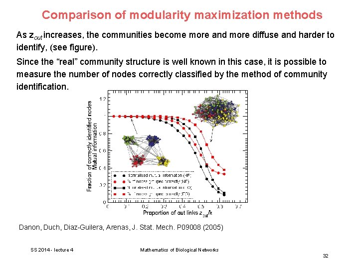
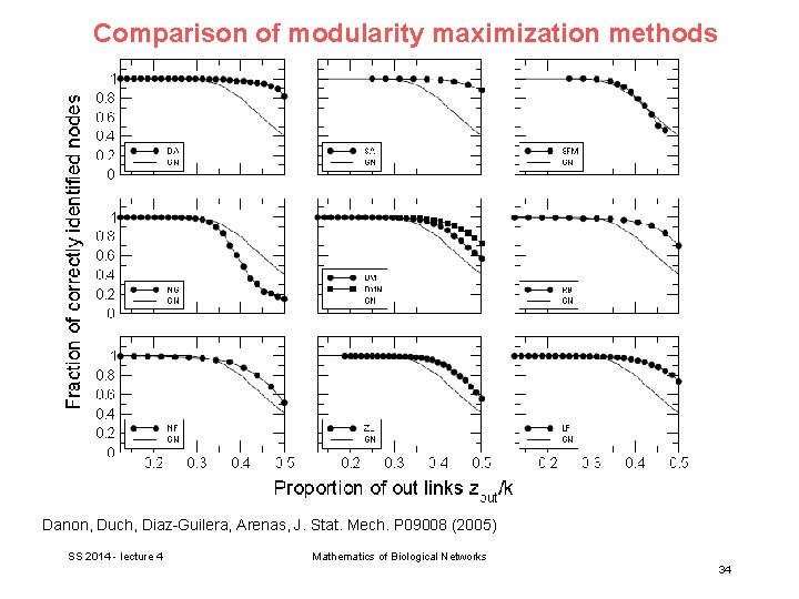
Comparison of modularity maximization methods One way to test the sensitivity of these methods is to see how well a particular method performs when applied to ad hoc networks with a well known, fixed community structure. Such networks are typically generated with n = 128 nodes, split into 4 communities containing 32 nodes each. Pairs of nodes belonging to the same community are linked with probability pin whereas pairs belonging to different communities are joined with probability pout. The value of pout is taken so that the average number of links a node has to members of any other community, zout, can be controlled. While pout (and therefore zout) is varied freely, the value of pin is chosen to keep the total average node degree, k constant, and set to 16. Danon, Duch, Diaz-Guilera, Arenas, J. Stat. Mech. P 09008 (2005) SS 2014 - lecture 4 Mathematics of Biological Networks 31

Comparison of modularity maximization methods As zout increases, the communities become more and more diffuse and harder to identify, (see figure). Since the “real” community structure is well known in this case, it is possible to measure the number of nodes correctly classified by the method of community identification. Danon, Duch, Diaz-Guilera, Arenas, J. Stat. Mech. P 09008 (2005) SS 2014 - lecture 4 Mathematics of Biological Networks 32

Other modularity maximization methods One of the most successful approaches is simulated annealing. The process begins with any initial partition of the nodes into communities. At each step, a node is chosen at random and moved to a different community, also chosen at random. If the change improves the modularity it is always accepted, otherwise it is accepted with a probability exp( Q/k. T). The simulation will start at high temperature T and is then slowly cooled down. Several improvements have been tested. Firstly, the algorithm is stopped periodically, or quenched, and Q is calculated for moving each node to every community that is not its own. Finally, the move corresponding to the largest value of Q is accepted. SS 2014 - lecture 4 Mathematics of Biological Networks 33

Comparison of modularity maximization methods Danon, Duch, Diaz-Guilera, Arenas, J. Stat. Mech. P 09008 (2005) SS 2014 - lecture 4 Mathematics of Biological Networks 34