V 19 Metabolic Networks Overview There exist different

V 19 Metabolic Networks - Overview There exist different levels of computational methods for describing metabolic networks: - stoichiometry/kinetics of classical biochemical pathways (glycolysis, TCA cycle, . . . - stoichiometric modelling (flux balance analysis): theoretical capabilities of an integrated cellular process, feasible metabolic flux distributions - automatic decomposition of metabolic networks (elementary nodes, extreme pathways. . . ) - kinetic modelling of coupled cellular pathways (E-Cell. . . ) General problem: lack of kinetic information on the dynamics and regulation of cellular metabolism 19. Lecture WS 2019/20 Bioinformatics III 1

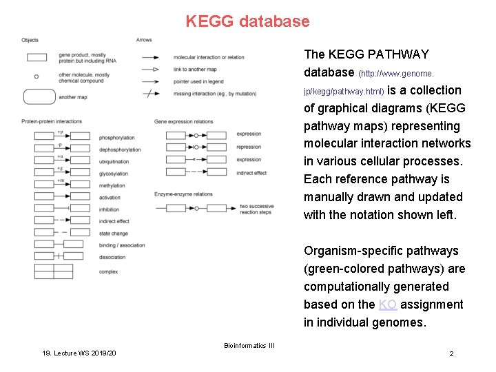
KEGG database The KEGG PATHWAY database (http: //www. genome. jp/kegg/pathway. html) is a collection of graphical diagrams (KEGG pathway maps) representing molecular interaction networks in various cellular processes. Each reference pathway is manually drawn and updated with the notation shown left. Organism-specific pathways (green-colored pathways) are computationally generated based on the KO assignment in individual genomes. 19. Lecture WS 2019/20 Bioinformatics III 2

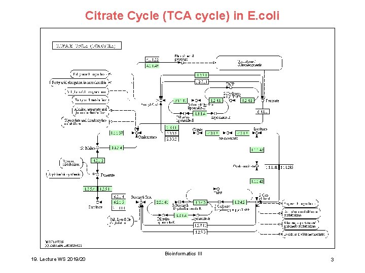
Citrate Cycle (TCA cycle) in E. coli 19. Lecture WS 2019/20 Bioinformatics III 3

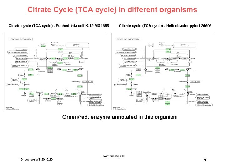
Citrate Cycle (TCA cycle) in different organisms Citrate cycle (TCA cycle) - Escherichia coli K-12 MG 1655 Citrate cycle (TCA cycle) - Helicobacter pylori 26695 Green/red: enzyme annotated in this organism 19. Lecture WS 2019/20 Bioinformatics III 4

Eco. Cyc Database E. coli genome contains 4. 7 million DNA bases. How can we characterize the functional complement of E. coli and according to what criteria can we compare the biochemical networks of two organisms? Eco. Cyc contains the metabolic map of E. coli defined as the set of all known pathways, reactions and enzymes of E. coli small-molecule metabolism. Analyze - the connectivity relationships of the metabolic network - its partitioning into pathways - enzyme activation and inhibition - repetition and multiplicity of elements such as enzymes, reactions, and substrates. Ouzonis, Karp, Genome Res. 10, 568 (2000) 19. Lecture WS 2019/20 Bioinformatics III 5

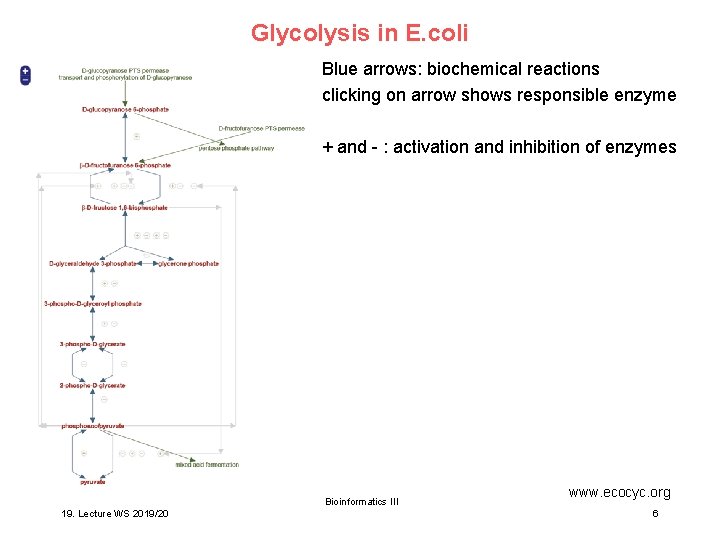
Glycolysis in E. coli Blue arrows: biochemical reactions clicking on arrow shows responsible enzyme + and - : activation and inhibition of enzymes Bioinformatics III 19. Lecture WS 2019/20 www. ecocyc. org 6

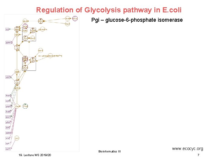
Regulation of Glycolysis pathway in E. coli Pgi – glucose-6 -phosphate isomerase Bioinformatics III 19. Lecture WS 2019/20 www. ecocyc. org 7

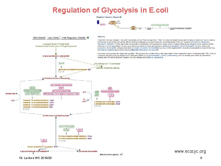
Regulation of Glycolysis in E. coli Bioinformatics III 19. Lecture WS 2019/20 www. ecocyc. org 8

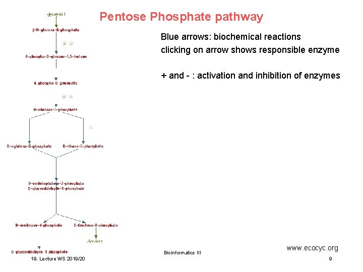
Pentose Phosphate pathway Blue arrows: biochemical reactions clicking on arrow shows responsible enzyme + and - : activation and inhibition of enzymes Bioinformatics III 19. Lecture WS 2019/20 www. ecocyc. org 9

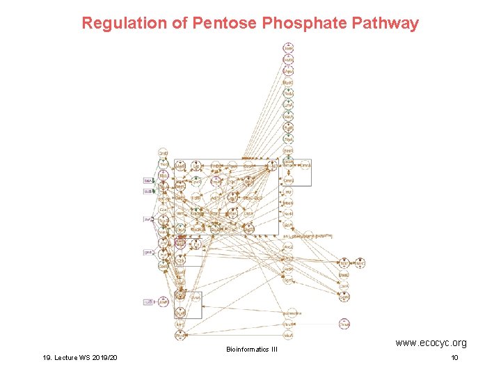
Regulation of Pentose Phosphate Pathway Bioinformatics III 19. Lecture WS 2019/20 www. ecocyc. org 10

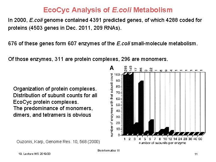
Eco. Cyc Analysis of E. coli Metabolism In 2000, E. coli genome contained 4391 predicted genes, of which 4288 coded for proteins (4503 genes in Dec. 2011, 209 RNAs). 676 of these genes form 607 enzymes of the E. coli small-molecule metabolism. Of those enzymes, 311 are protein complexes, 296 are monomers. Organization of protein complexes. Distribution of subunit counts for all Eco. Cyc protein complexes. The predominance of monomers, dimers, and tetramers is obvious Ouzonis, Karp, Genome Res. 10, 568 (2000) 19. Lecture WS 2019/20 Bioinformatics III 11

Reactions Eco. Cyc describes 905 metabolic reactions that are catalyzed by E. coli. (1991 in Dec. 2011) Of these reactions, 161 are not involved in small-molecule metabolism, e. g. they participate in macromolecule metabolism such as DNA replication and t. RNA charging. Of the remaining 744 reactions, 569 have been assigned to at least one pathway. Ouzonis, Karp, Genome Res. 10, 568 (2000) 19. Lecture WS 2019/20 Bioinformatics III 12

Reactions The number of reactions (744) and the number of enzymes (607) differ. . . WHY? ? (1) there is no one-to-one mapping between enzymes and reactions – some enzymes catalyze multiple reactions, and some reactions are catalyzed by multiple enzymes. (2) for some reactions known to be catalyzed by E. coli, the enzyme has not yet been identified. Ouzonis, Karp, Genome Res. 10, 568 (2000) 19. Lecture WS 2019/20 Bioinformatics III 13

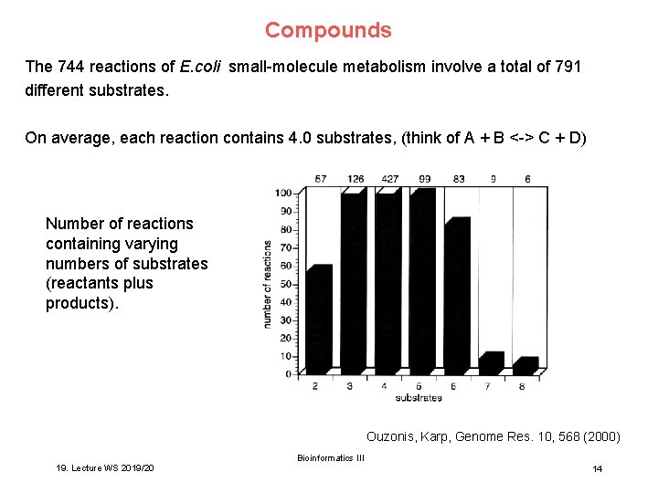
Compounds The 744 reactions of E. coli small-molecule metabolism involve a total of 791 different substrates. On average, each reaction contains 4. 0 substrates, (think of A + B <-> C + D) Number of reactions containing varying numbers of substrates (reactants plus products). Ouzonis, Karp, Genome Res. 10, 568 (2000) 19. Lecture WS 2019/20 Bioinformatics III 14

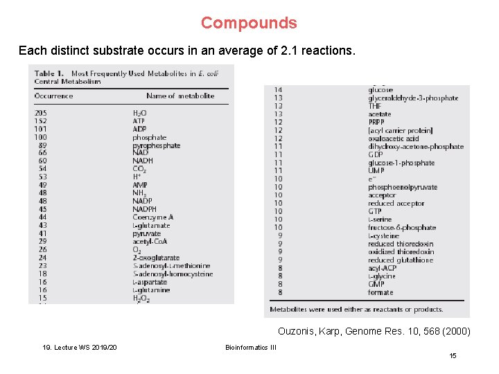
Compounds Each distinct substrate occurs in an average of 2. 1 reactions. Ouzonis, Karp, Genome Res. 10, 568 (2000) 19. Lecture WS 2019/20 Bioinformatics III 15

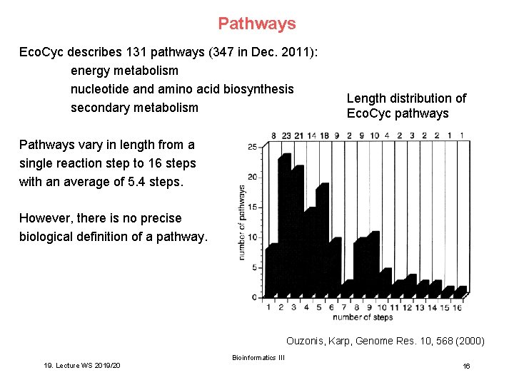
Pathways Eco. Cyc describes 131 pathways (347 in Dec. 2011): energy metabolism nucleotide and amino acid biosynthesis secondary metabolism Length distribution of Eco. Cyc pathways Pathways vary in length from a single reaction step to 16 steps with an average of 5. 4 steps. However, there is no precise biological definition of a pathway. Ouzonis, Karp, Genome Res. 10, 568 (2000) 19. Lecture WS 2019/20 Bioinformatics III 16

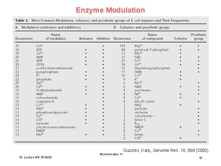
Enzyme Modulation An enzymatic reaction is a type of Eco. Cyc object that represents the pairing of an enzyme with a reaction catalyzed by that enzyme. Eco. Cyc contains extensive information on the modulation of E. coli enzymes with respect to particular reactions: - activators and inhibitors of the enzyme, - cofactors required by the enzyme - alternative substrates that the enzyme will accept. Of the 805 enzymatic-reaction objects within Eco. Cyc, physiologically relevant activators are known for 22, physiologically relevant inhibitors are known for 80. 327 (almost half) require a cofactor or prosthetic group. Ouzonis, Karp, Genome Res. 10, 568 (2000) 19. Lecture WS 2019/20 Bioinformatics III 17

Enzyme Modulation 19. Lecture WS 2019/20 Bioinformatics III Ouzonis, Karp, Genome Res. 10, 568 (2000) 18

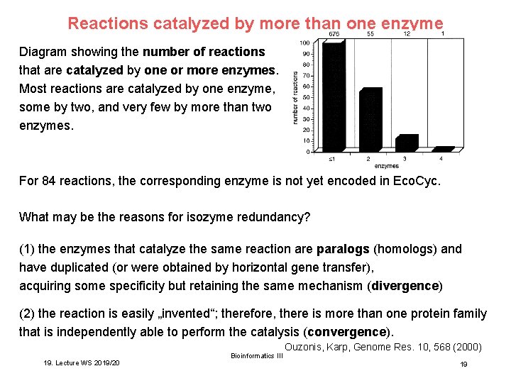
Reactions catalyzed by more than one enzyme Diagram showing the number of reactions that are catalyzed by one or more enzymes. Most reactions are catalyzed by one enzyme, some by two, and very few by more than two enzymes. For 84 reactions, the corresponding enzyme is not yet encoded in Eco. Cyc. What may be the reasons for isozyme redundancy? (1) the enzymes that catalyze the same reaction are paralogs (homologs) and have duplicated (or were obtained by horizontal gene transfer), acquiring some specificity but retaining the same mechanism (divergence) (2) the reaction is easily „invented“; therefore, there is more than one protein family that is independently able to perform the catalysis (convergence). 19. Lecture WS 2019/20 Bioinformatics III Ouzonis, Karp, Genome Res. 10, 568 (2000) 19

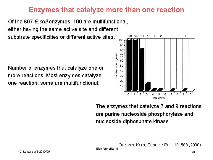
Enzymes that catalyze more than one reaction Of the 607 E. coli enzymes, 100 are multifunctional, either having the same active site and different substrate specificities or different active sites. Number of enzymes that catalyze one or more reactions. Most enzymes catalyze one reaction; some are multifunctional. The enzymes that catalyze 7 and 9 reactions are purine nucleoside phosphorylase and nucleoside diphosphate kinase. 19. Lecture WS 2019/20 Bioinformatics III Ouzonis, Karp, Genome Res. 10, 568 (2000) 20

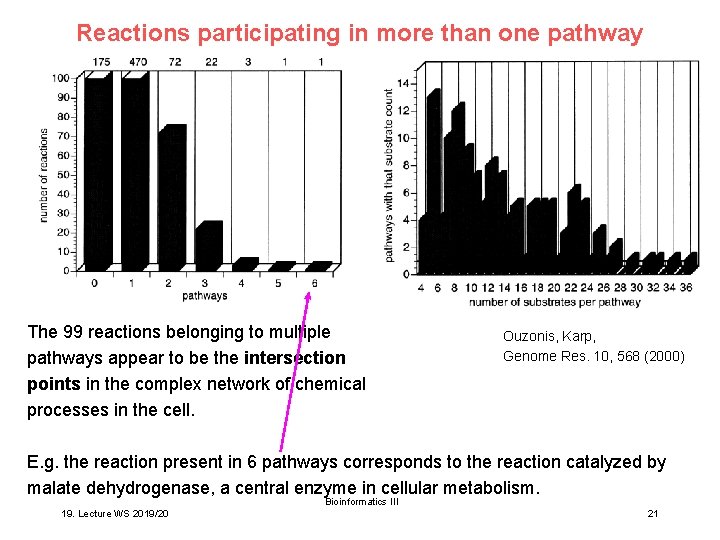
Reactions participating in more than one pathway The 99 reactions belonging to multiple pathways appear to be the intersection points in the complex network of chemical processes in the cell. Ouzonis, Karp, Genome Res. 10, 568 (2000) E. g. the reaction present in 6 pathways corresponds to the reaction catalyzed by malate dehydrogenase, a central enzyme in cellular metabolism. Bioinformatics III 19. Lecture WS 2019/20 21

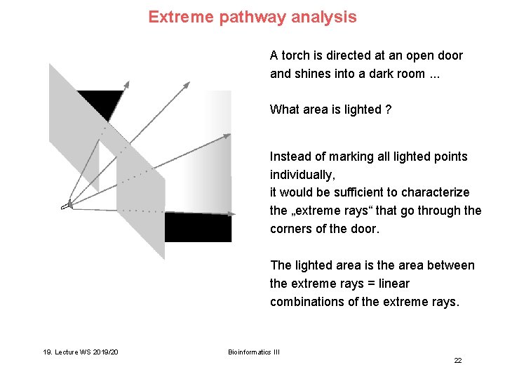
Extreme pathway analysis A torch is directed at an open door and shines into a dark room. . . What area is lighted ? Instead of marking all lighted points individually, it would be sufficient to characterize the „extreme rays“ that go through the corners of the door. The lighted area is the area between the extreme rays = linear combinations of the extreme rays. 19. Lecture WS 2019/20 Bioinformatics III 22

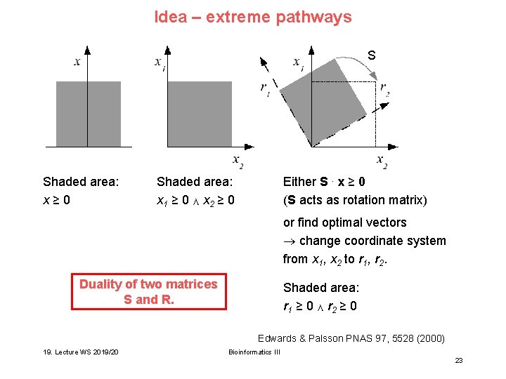
Idea – extreme pathways S Shaded area: x ≥ 0 Shaded area: x 1 ≥ 0 ∧ x 2 ≥ 0 Either S. x ≥ 0 (S acts as rotation matrix) or find optimal vectors change coordinate system from x 1, x 2 to r 1, r 2. Duality of two matrices S and R. Shaded area: r 1 ≥ 0 ∧ r 2 ≥ 0 Edwards & Palsson PNAS 97, 5528 (2000) 19. Lecture WS 2019/20 Bioinformatics III 23

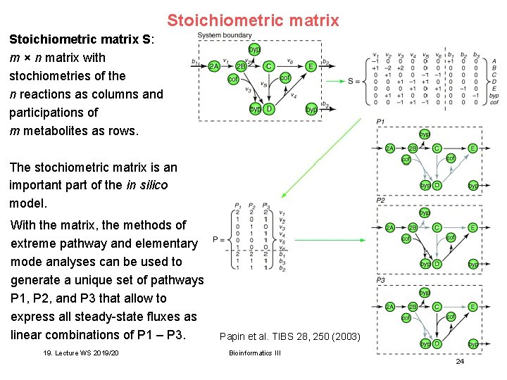
Stoichiometric matrix S: m × n matrix with stochiometries of the n reactions as columns and participations of m metabolites as rows. The stochiometric matrix is an important part of the in silico model. With the matrix, the methods of extreme pathway and elementary mode analyses can be used to generate a unique set of pathways P 1, P 2, and P 3 that allow to express all steady-state fluxes as linear combinations of P 1 – P 3. 19. Lecture WS 2019/20 Papin et al. TIBS 28, 250 (2003) Bioinformatics III 24

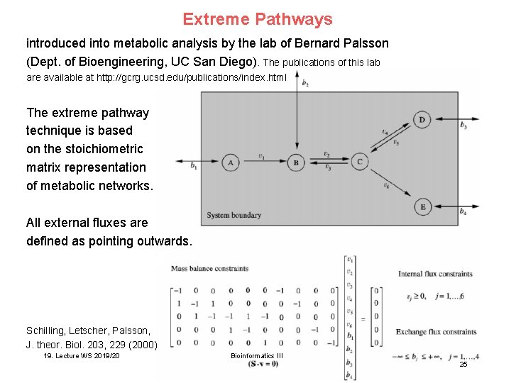
Extreme Pathways introduced into metabolic analysis by the lab of Bernard Palsson (Dept. of Bioengineering, UC San Diego). The publications of this lab are available at http: //gcrg. ucsd. edu/publications/index. html The extreme pathway technique is based on the stoichiometric matrix representation of metabolic networks. All external fluxes are defined as pointing outwards. Schilling, Letscher, Palsson, J. theor. Biol. 203, 229 (2000) 19. Lecture WS 2019/20 Bioinformatics III 25

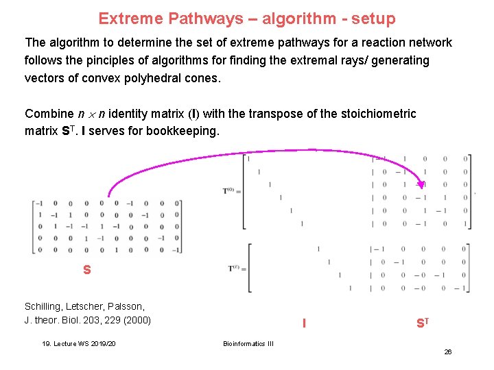
Extreme Pathways – algorithm - setup The algorithm to determine the set of extreme pathways for a reaction network follows the pinciples of algorithms for finding the extremal rays/ generating vectors of convex polyhedral cones. Combine n n identity matrix (I) with the transpose of the stoichiometric matrix ST. I serves for bookkeeping. S Schilling, Letscher, Palsson, J. theor. Biol. 203, 229 (2000) 19. Lecture WS 2019/20 I ST Bioinformatics III 26

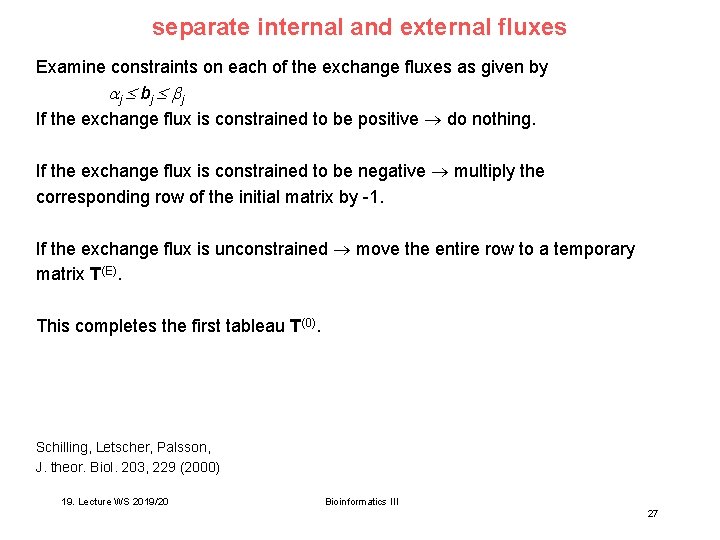
separate internal and external fluxes Examine constraints on each of the exchange fluxes as given by j bj j If the exchange flux is constrained to be positive do nothing. If the exchange flux is constrained to be negative multiply the corresponding row of the initial matrix by -1. If the exchange flux is unconstrained move the entire row to a temporary matrix T(E). This completes the first tableau T(0). Schilling, Letscher, Palsson, J. theor. Biol. 203, 229 (2000) 19. Lecture WS 2019/20 Bioinformatics III 27

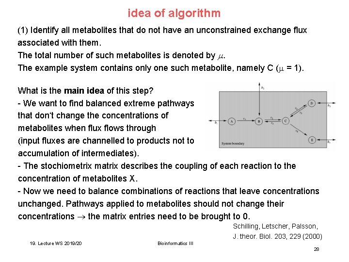
idea of algorithm (1) Identify all metabolites that do not have an unconstrained exchange flux associated with them. The total number of such metabolites is denoted by . The example system contains only one such metabolite, namely C ( = 1). What is the main idea of this step? - We want to find balanced extreme pathways that don‘t change the concentrations of metabolites when flux flows through (input fluxes are channelled to products not to accumulation of intermediates). - The stochiometrix matrix describes the coupling of each reaction to the concentration of metabolites X. - Now we need to balance combinations of reactions that leave concentrations unchanged. Pathways applied to metabolites should not change their concentrations the matrix entries need to be brought to 0. Schilling, Letscher, Palsson, J. theor. Biol. 203, 229 (2000) 19. Lecture WS 2019/20 Bioinformatics III 28

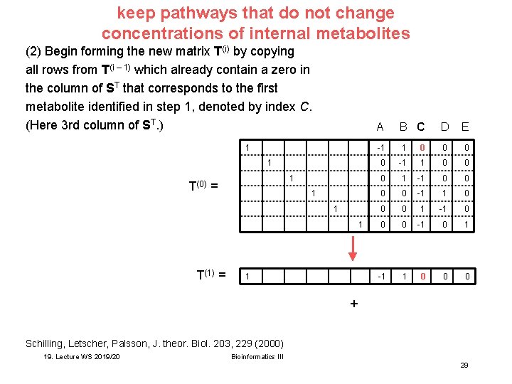
keep pathways that do not change concentrations of internal metabolites (2) Begin forming the new matrix T(i) by copying all rows from T(i – 1) which already contain a zero in the column of ST that corresponds to the first metabolite identified in step 1, denoted by index C. (Here 3 rd column of ST. ) A B C D E 1 1 1 T(0) = 1 1 1 T(1) = 1 -1 1 0 0 0 0 -1 1 0 0 0 1 -1 0 0 0 -1 0 1 -1 1 0 0 0 + Schilling, Letscher, Palsson, J. theor. Biol. 203, 229 (2000) 19. Lecture WS 2019/20 Bioinformatics III 29

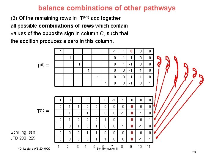
balance combinations of other pathways (3) Of the remaining rows in T(i-1) add together all possible combinations of rows which contain values of the opposite sign in column C, such that the addition produces a zero in this column. 1 -1 1 0 0 0 0 -1 1 0 0 0 1 -1 0 0 -1 0 1 1 1 T(0) = 1 1 T(1) = Schilling, et al. JTB 203, 229 19. Lecture WS 2019/20 1 0 0 0 -1 1 0 0 0 0 1 0 0 0 -1 0 0 0 1 0 -1 0 0 1 0 -1 0 0 1 1 0 0 0 -1 1 1 2 3 4 5 6 7 8 9 10 11 Bioinformatics III 30

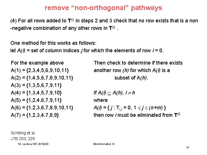
remove “non-orthogonal” pathways (4) For all rows added to T(i) in steps 2 and 3 check that no row exists that is a non -negative combination of any other rows in T(i). One method for this works as follows: let A(i) = set of column indices j for which the elements of row i = 0. For the example above A(1) = {2, 3, 4, 5, 6, 9, 10, 11} A(2) = {1, 4, 5, 6, 7, 8, 9, 10, 11} A(3) = {1, 3, 5, 6, 7, 9, 11} A(4) = {1, 3, 4, 5, 7, 9, 10} A(5) = {1, 2, 4, 6, 7, 9, 11} A(6) = {1, 2, 3, 6, 7, 8, 9, 10, 11} A(7) = {1, 2, 3, 4, 7, 8, 9} Then check to determine if there exists another row (h) for which A(i) is a subset of A(h). If A(i) A(h), i h where A(i) = { j : Ti, j = 0, 1 j (n+m) } then row i must be eliminated from T(i) Schilling et al. JTB 203, 229 19. Lecture WS 2019/20 Bioinformatics III 31

repeat steps for all internal metabolites (5) With the formation of T(i) complete steps 2 – 4 for all of the metabolites that do not have an unconstrained exchange flux operating on the metabolite, incrementing i by one up to . The final tableau will be T( ). Note that the number of rows in T( ) will be equal to k, the number of extreme pathways. Schilling et al. JTB 203, 229 19. Lecture WS 2019/20 Bioinformatics III 32

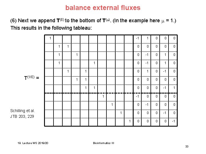
balance external fluxes (6) Next we append T(E) to the bottom of T( ). (In the example here = 1. ) This results in the following tableau: 1 1 -1 1 0 0 0 0 0 -1 0 1 0 1 0 -1 0 0 0 0 0 -1 1 -1 0 0 0 -1 0 0 0 -1 1 1 1 T(1/E) = 1 1 1 Schilling et al. JTB 203, 229 1 1 19. Lecture WS 2019/20 Bioinformatics III 33

balance external fluxes (7) Starting in the n+1 column (or the first non-zero column on the right side), if Ti, (n+1) 0 then add the corresponding non-zero row from T(E) to row i so as to produce 0 in the n+1 -th column. This is done by simply multiplying the corresponding row in T(E) by Ti, (n+1) and adding this row to row i. Repeat this procedure for each of the rows in the upper portion of the tableau so as to create zeros in the entire upper portion of the (n+1) column. When finished, remove the row in T(E) corresponding to the exchange flux for the metabolite just balanced. Schilling et al. JTB 203, 229 19. Lecture WS 2019/20 Bioinformatics III 34

balance external fluxes (8) Follow the same procedure as in step (7) for each of the columns on the right side of the tableau containing non-zero entries. (In our example we need to perform step (7) for every column except the middle column of the right side which correponds to metabolite C. ) The final tableau T(final) will contain the transpose of the matrix P containing the extreme pathways in place of the original identity matrix. Schilling et al. JTB 203, 229 19. Lecture WS 2019/20 Bioinformatics III 35

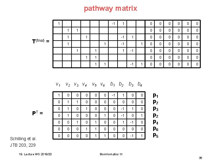
pathway matrix 1 -1 1 T(final) = 1 -1 1 PT = Schilling et al. JTB 203, 229 19. Lecture WS 2019/20 1 1 -1 1 1 v 2 v 3 v 4 1 -1 1 1 v 5 v 6 -1 b 2 1 0 0 0 0 0 0 0 0 0 0 0 b 3 b 4 1 0 0 0 -1 1 0 0 0 1 0 0 0 -1 1 0 0 0 1 0 -1 0 1 0 0 1 -1 0 0 1 1 0 0 0 0 0 1 1 0 0 -1 1 p 7 p 3 p 2 p 4 p 6 p 5 Bioinformatics III 36

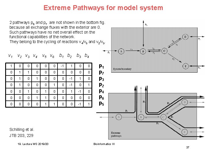
Extreme Pathways for model system 2 pathways p 6 and p 7 are not shown in the bottom fig. because all exchange fluxes with the exterior are 0. Such pathways have no net overall effect on the functional capabilities of the network. They belong to the cycling of reactions v 4/v 5 and v 2/v 3. v 1 v 2 v 3 v 4 v 5 v 6 b 1 b 2 b 3 b 4 1 0 0 0 -1 1 0 0 0 1 0 0 0 -1 1 0 0 0 1 0 -1 0 1 0 0 1 -1 0 0 1 1 0 0 0 0 0 1 1 0 0 -1 1 p 7 p 3 p 2 p 4 p 6 p 5 Schilling et al. JTB 203, 229 19. Lecture WS 2019/20 Bioinformatics III 37

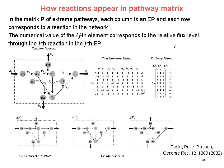
How reactions appear in pathway matrix In the matrix P of extreme pathways, each column is an EP and each row corresponds to a reaction in the network. The numerical value of the i, j-th element corresponds to the relative flux level through the i-th reaction in the j-th EP. 19. Lecture WS 2019/20 Bioinformatics III Papin, Price, Palsson, Genome Res. 12, 1889 (2002) 38

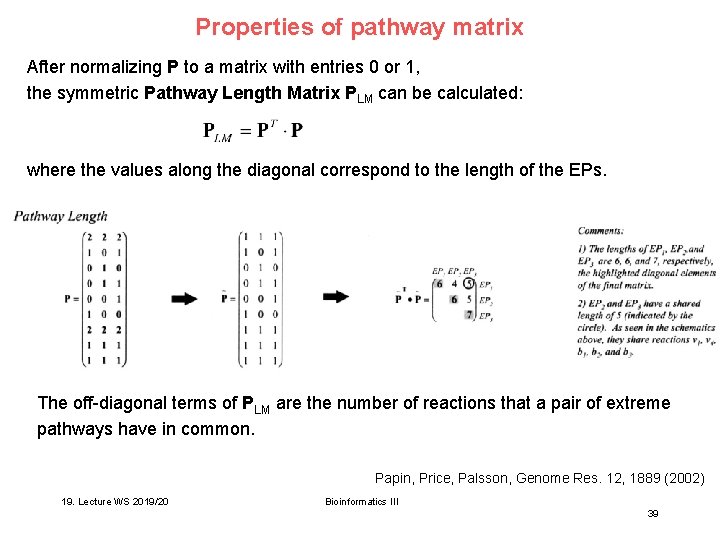
Properties of pathway matrix After normalizing P to a matrix with entries 0 or 1, the symmetric Pathway Length Matrix PLM can be calculated: where the values along the diagonal correspond to the length of the EPs. The off-diagonal terms of PLM are the number of reactions that a pair of extreme pathways have in common. Papin, Price, Palsson, Genome Res. 12, 1889 (2002) 19. Lecture WS 2019/20 Bioinformatics III 39

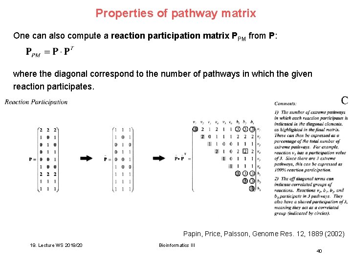
Properties of pathway matrix One can also compute a reaction participation matrix PPM from P: where the diagonal correspond to the number of pathways in which the given reaction participates. Papin, Price, Palsson, Genome Res. 12, 1889 (2002) 19. Lecture WS 2019/20 Bioinformatics III 40

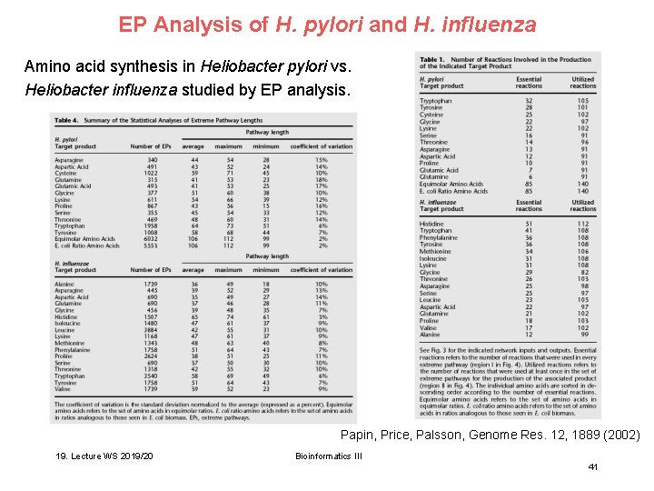
EP Analysis of H. pylori and H. influenza Amino acid synthesis in Heliobacter pylori vs. Heliobacter influenza studied by EP analysis. Papin, Price, Palsson, Genome Res. 12, 1889 (2002) 19. Lecture WS 2019/20 Bioinformatics III 41

Summary – Extreme Pathways Extreme Pathway Analysis is a standard technique for analysis of metabolic networks. Number of EPs can become extremely large – hard to interpret. EP is an excellent basis for studying systematic effects of reaction cut sets. It will be very important to consider the interplay of metabolic and regulatory networks. 19. Lecture WS 2019/20 Bioinformatics III 42