V 17 The Double Description method Theoretical framework

V 17 The Double Description method: Theoretical framework behind EFM and EP / Integration Algorithms in „Combinatorics and Computer Science Vol. 1120“ edited by Deza, Euler, Manoussakis, Springer, 1996: 91 17. Lecture WS 2015/16 Bioinformatics III 1

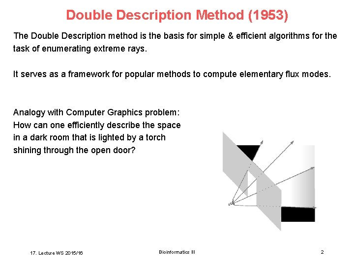
Double Description Method (1953) The Double Description method is the basis for simple & efficient algorithms for the task of enumerating extreme rays. It serves as a framework for popular methods to compute elementary flux modes. Analogy with Computer Graphics problem: How can one efficiently describe the space in a dark room that is lighted by a torch shining through the open door? 17. Lecture WS 2015/16 Bioinformatics III 2

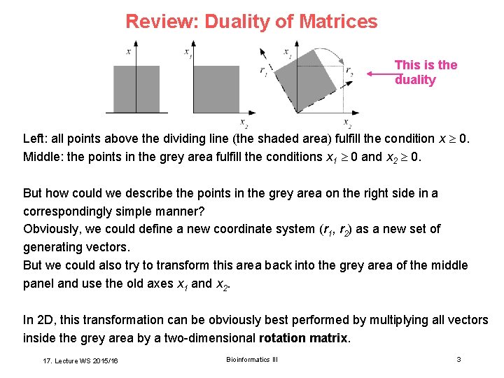
Review: Duality of Matrices This is the duality Left: all points above the dividing line (the shaded area) fulfill the condition x 0. Middle: the points in the grey area fulfill the conditions x 1 0 and x 2 0. But how could we describe the points in the grey area on the right side in a correspondingly simple manner? Obviously, we could define a new coordinate system (r 1, r 2) as a new set of generating vectors. But we could also try to transform this area back into the grey area of the middle panel and use the old axes x 1 and x 2. In 2 D, this transformation can be obviously best performed by multiplying all vectors inside the grey area by a two-dimensional rotation matrix. 17. Lecture WS 2015/16 Bioinformatics III 3

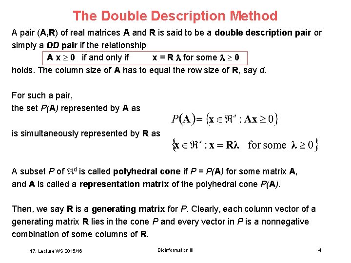
The Double Description Method A pair (A, R) of real matrices A and R is said to be a double description pair or simply a DD pair if the relationship A x 0 if and only if x = R for some 0 holds. The column size of A has to equal the row size of R, say d. For such a pair, the set P(A) represented by A as is simultaneously represented by R as A subset P of d is called polyhedral cone if P = P(A) for some matrix A, and A is called a representation matrix of the polyhedral cone P(A). Then, we say R is a generating matrix for P. Clearly, each column vector of a generating matrix R lies in the cone P and every vector in P is a nonnegative combination of some columns of R. 17. Lecture WS 2015/16 Bioinformatics III 4

The Double Description Method Theorem 1 (Minkowski‘s Theorem for Polyhedral Cones) For any m n real matrix A, there exists some d m real matrix R such that (A, R) is a DD pair, or in other words, the cone P(A) is generated by R. The theorem states that every polyhedral cone admits a generating matrix. The nontriviality comes from the fact that the row size of R is finite. If we allow an infinite size, there is a trivial generating matrix consisting of all vectors in the cone. Also the converse is true: Theorem 2 (Weyl‘s Theorem for Polyhedral Cones) For any d n real matrix R, there exists some m d real matrix A such that (A, R) is a DD pair, or in other words, the set generated by R is the cone P(A). 17. Lecture WS 2015/16 Bioinformatics III 5

The Double Description Method Task: how does one construct a matrix R from a given matrix A, and the converse? These two problems are computationally equivalent. Farkas‘ Lemma shows that (A, R) is a DD pair if and only if (RT, AT) is a DD pair. A more appropriate formulation of the problem is to require the minimality of R: find a matrix R such that no proper submatrix is generating P(A). A minimal set of generators is unique up to positive scaling when we assume the regularity condition that the cone is pointed, i. e. the origin is an extreme point of P(A). Geometrically, the columns of a minimal generating matrix are in 1 -to-1 correspondence with the extreme rays of P. Thus the problem is also known as the extreme ray enumeration problem. No efficient (polynomial) algorithm is known for the general problem. 17. Lecture WS 2015/16 Bioinformatics III 6

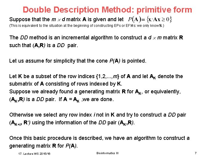
Double Description Method: primitive form Suppose that the m d matrix A is given and let (This is equivalent to the situation at the beginning of constructing EPs or EFMs: we only know S. ) The DD method is an incremental algorithm to construct a d m matrix R such that (A, R) is a DD pair. Let us assume for simplicity that the cone P(A) is pointed. Let K be a subset of the row indices {1, 2, . . . , m} of A and let AK denote the submatrix of A consisting of rows indexed by K. Suppose we already found a generating matrix R for AK, or equivalently, (AK, R) is a DD pair. If A = AK , we are done. Otherwise we select any row index i not in K and try to construct a DD pair (AK+i, R‘) using the information of the DD pair (AK, R). Once this basic procedure is described, we have an algorithm to construct a generating matrix R for P(A). 17. Lecture WS 2015/16 Bioinformatics III 7

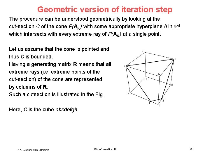
Geometric version of iteration step The procedure can be understood geometrically by looking at the cut-section C of the cone P(AK) with some appropriate hyperplane h in d which intersects with every extreme ray of P(AK) at a single point. Let us assume that the cone is pointed and thus C is bounded. Having a generating matrix R means that all extreme rays (i. e. extreme points of the cut-section) of the cone are represented by columns of R. Such a cutsection is illustrated in the Fig. Here, C is the cube abcdefgh. 17. Lecture WS 2015/16 Bioinformatics III 8

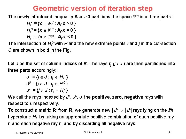
Geometric version of iteration step The newly introduced inequality Ai x 0 partitions the space d into three parts: Hi+ = {x d : Ai x > 0 } Hi 0 = {x d : Ai x = 0 } Hi- = {x d : Ai x < 0 } The intersection of Hi 0 with P and the new extreme points i and j in the cut-section C are shown in bold in the Fig. Let J be the set of column indices of R. The rays rj (j J ) are then partitioned into three parts accordingly: J+ = {j J : rj Hi+ } J 0 = {j J : rj Hi 0 } J- = {j J : rj Hi- } We call the rays indexed by J+, J 0, J- the positive, zero, negative rays with respect to i, respectively. To construct a matrix R‘ from R, we generate new | J+| | J-| rays lying on the ith hyperplane Hi 0 by taking an appropriate positive combination of each positive ray rj and each negative ray rj‘ and by discarding all negative rays. 17. Lecture WS 2015/16 Bioinformatics III 9

Geometric version of iteration step The following lemma ensures that we have a DD pair (AK+i , R‘), and provides the key procedure for the most primitive version of the DD method. Lemma 3 Let (AK, R) be a DD pair and let i be a row index of A not in K. Then the pair (AK+i , R‘) is a DD pair, where R‘ is the d |J‘ | matrix with column vectors rj (j J‘) defined by J‘ = J+ J 0 (J+ J-), and rjj‘ = (Ai rj) rj‘ – (Ai rj‘) rj for each (j, j‘) J+ JProof omitted. 17. Lecture WS 2015/16 Bioinformatics III 10

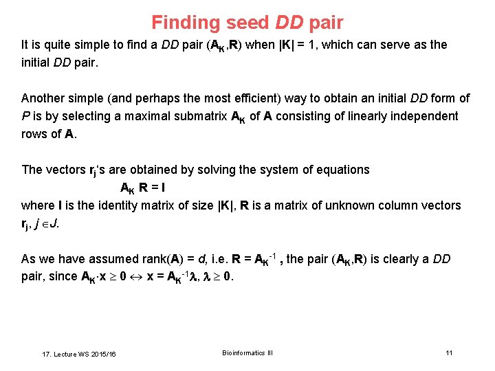
Finding seed DD pair It is quite simple to find a DD pair (AK, R) when |K| = 1, which can serve as the initial DD pair. Another simple (and perhaps the most efficient) way to obtain an initial DD form of P is by selecting a maximal submatrix AK of A consisting of linearly independent rows of A. The vectors rj‘s are obtained by solving the system of equations AK R = I where I is the identity matrix of size |K|, R is a matrix of unknown column vectors rj, j J. As we have assumed rank(A) = d, i. e. R = AK-1 , the pair (AK, R) is clearly a DD pair, since AK x 0 x = AK-1 , 0. 17. Lecture WS 2015/16 Bioinformatics III 11

Primitive algorithm for Double. Description. Method This algorithm is very primitive, and the straightforward implementation will be quite useless, because the size of J increases extremely fast. This is because many vectors rjj‘ generated by the algorithm (defined in Lemma 3) are unnessary. We need to avoid generating redundant vectors! To avoid generating redundant vectors, we will use the zero set or active set Z(x) which is the set of inequality indices satisfied by x in P(A) with equality. Noting A i • the ith row of A, Z(x) = {i : A i • x = 0} 17. Lecture WS 2015/16 Bioinformatics III 12

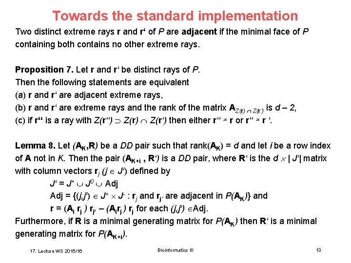
Towards the standard implementation Two distinct extreme rays r and r‘ of P are adjacent if the minimal face of P containing both contains no other extreme rays. Proposition 7. Let r and r‘ be distinct rays of P. Then the following statements are equivalent (a) r and r‘ are adjacent extreme rays, (b) r and r‘ are extreme rays and the rank of the matrix AZ(r) Z(r‘) is d – 2, (c) if r‘‘ is a ray with Z(r‘‘) Z(r‘) then either r‘‘ ≃ r or r‘‘ ≃ r ‘. Lemma 8. Let (AK, R) be a DD pair such that rank(AK) = d and let i be a row index of A not in K. Then the pair (AK+i , R‘) is a DD pair, where R‘ is the d | J‘| matrix with column vectors rj (j J‘) defined by J‘ = J+ J 0 Adj = {(j, j‘) J+ J- : rj and rj‘ are adjacent in P(AK)} and r = (Ai rj ) rj‘ – (Airj ) rj for each (j, j‘) Adj. Furthermore, if R is a minimal generating matrix for P(AK) then R‘ is a minimal generating matrix for P(AK+i). 17. Lecture WS 2015/16 Bioinformatics III 13

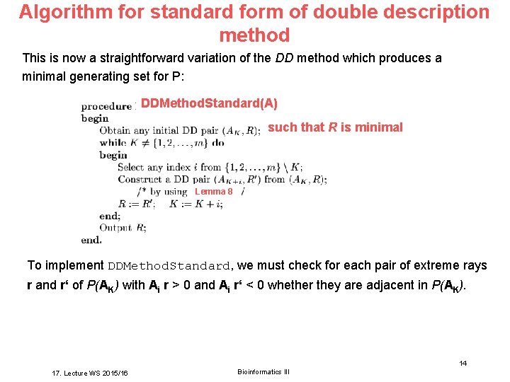
Algorithm for standard form of double description method This is now a straightforward variation of the DD method which produces a minimal generating set for P: DDMethod. Standard(A) such that R is minimal Lemma 8 To implement DDMethod. Standard, we must check for each pair of extreme rays r and r‘ of P(AK) with Ai r > 0 and Ai r‘ < 0 whether they are adjacent in P(AK). Bioinformatics III 14 17. Lecture WS 2015/16 Bioinformatics III

V 17 – second part Dynamic Modelling: Rate Equations + Stochastic Propagation 17. Lecture WS 2015/16 Bioinformatics III 15

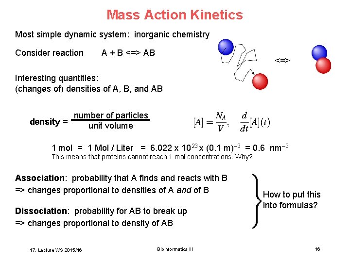
Mass Action Kinetics Most simple dynamic system: inorganic chemistry Consider reaction A + B <=> AB <=> Interesting quantities: (changes of) densities of A, B, and AB number of particles density = unit volume 1 mol = 1 Mol / Liter = 6. 022 x 1023 x (0. 1 m)– 3 = 0. 6 nm– 3 This means that proteins cannot reach 1 mol concentrations. Why? Association: probability that A finds and reacts with B => changes proportional to densities of A and of B Dissociation: probability for AB to break up => changes proportional to density of AB 17. Lecture WS 2015/16 Bioinformatics III How to put this into formulas? 16

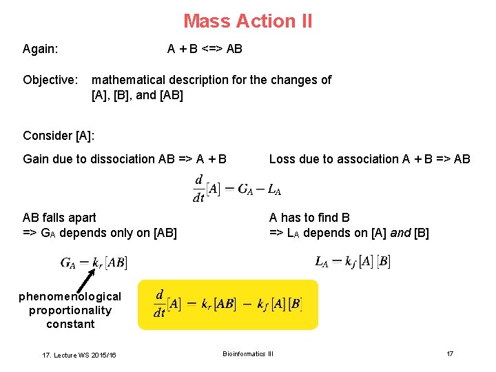
Mass Action II Again: Objective: A + B <=> AB mathematical description for the changes of [A], [B], and [AB] Consider [A]: Gain due to dissociation AB => A + B Loss due to association A + B => AB AB falls apart => GA depends only on [AB] A has to find B => LA depends on [A] and [B] phenomenological proportionality constant 17. Lecture WS 2015/16 Bioinformatics III 17

Mass Action !!! A + B <=> AB For [A]: we just found: For [B]: for symmetry reasons For [AB]: exchange gain and loss with [A](t 0), [B](t 0), and [AB](t 0) => complete description of the system time course = initial conditions + dynamics 17. Lecture WS 2015/16 Bioinformatics III 18

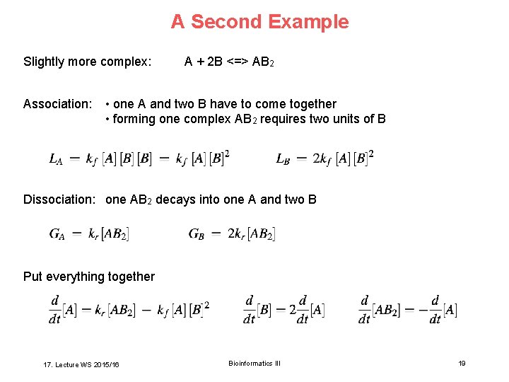
A Second Example Slightly more complex: Association: A + 2 B <=> AB 2 • one A and two B have to come together • forming one complex AB 2 requires two units of B Dissociation: one AB 2 decays into one A and two B Put everything together 17. Lecture WS 2015/16 Bioinformatics III 19

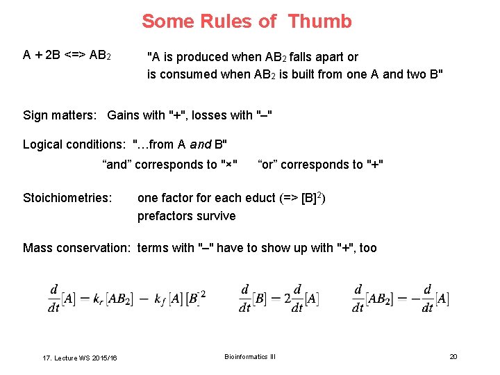
Some Rules of Thumb A + 2 B <=> AB 2 "A is produced when AB 2 falls apart or is consumed when AB 2 is built from one A and two B" Sign matters: Gains with "+", losses with "–" Logical conditions: "…from A and B" “and” corresponds to "×" Stoichiometries: “or” corresponds to "+" one factor for each educt (=> [B]2) prefactors survive Mass conservation: terms with "–" have to show up with "+", too 17. Lecture WS 2015/16 Bioinformatics III 20

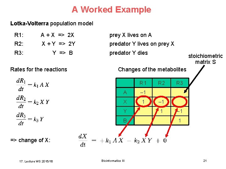
A Worked Example Lotka-Volterra population model R 1: A + X => 2 X prey X lives on A R 2: X + Y => 2 Y predator Y lives on prey X R 3: Y => B Rates for the reactions predator Y dies stoichiometric matrix S Changes of the metabolites R 1 A – 1 X 1 Y B R 2 R 3 – 1 1 => change of X: 17. Lecture WS 2015/16 Bioinformatics III 21

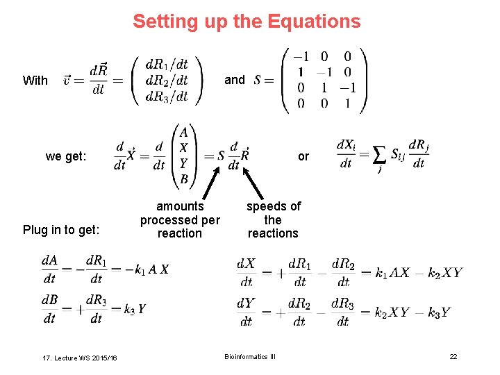
Setting up the Equations and With we get: Plug in to get: 17. Lecture WS 2015/16 or amounts processed per reaction speeds of the reactions Bioinformatics III 22

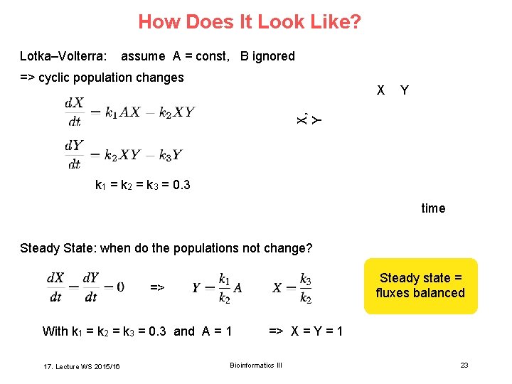
How Does It Look Like? Lotka–Volterra: assume A = const, B ignored => cyclic population changes Y X, Y X k 1 = k 2 = k 3 = 0. 3 time Steady State: when do the populations not change? Steady state = fluxes balanced => With k 1 = k 2 = k 3 = 0. 3 and A = 1 17. Lecture WS 2015/16 => X = Y = 1 Bioinformatics III 23

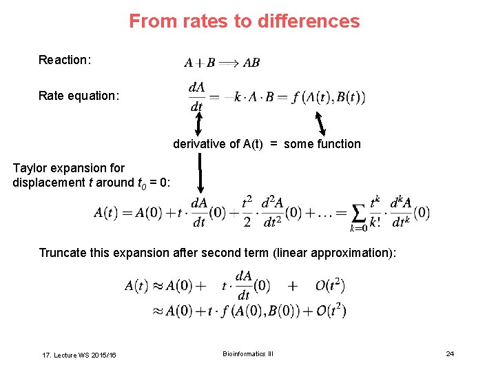
From rates to differences Reaction: Rate equation: derivative of A(t) = some function Taylor expansion for displacement t around t 0 = 0: Truncate this expansion after second term (linear approximation): 17. Lecture WS 2015/16 Bioinformatics III 24

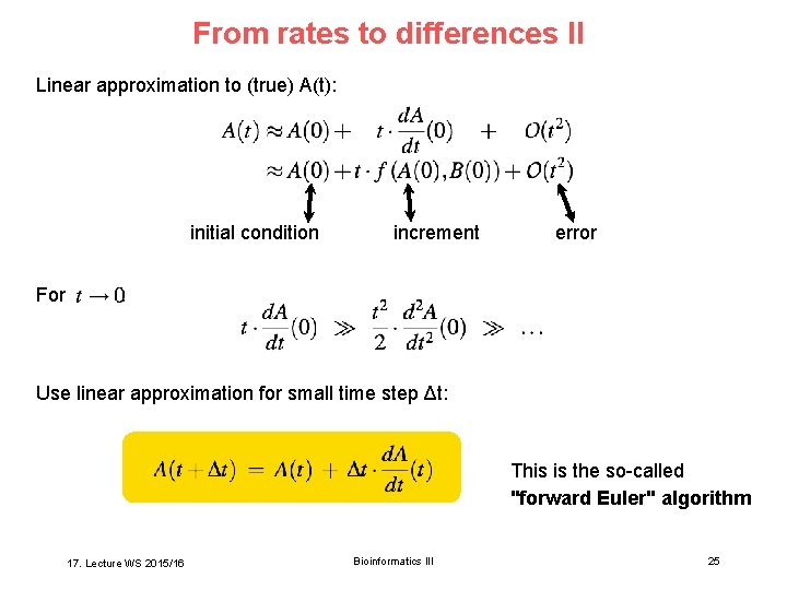
From rates to differences II Linear approximation to (true) A(t): initial condition For increment error : Use linear approximation for small time step Δt: This is the so-called "forward Euler" algorithm 17. Lecture WS 2015/16 Bioinformatics III 25

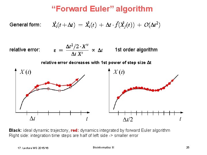
“Forward Euler” algorithm General form: relative error: 1 st order algorithm relative error decreases with 1 st power of step size Δt Black: ideal dynamic trajectory, red: dynamics integrated by forward Euler algorithm Right side: integration time steps are half of left side -> smaller error 17. Lecture WS 2015/16 Bioinformatics III 26

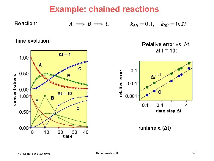
Example: chained reactions Reaction: Time evolution: Relative error vs. Δt at t = 10: Δt = 1 A, B C relative error concentrations A B Δt = 10 C C time step Δt runtime α (Δt)– 1 time 17. Lecture WS 2015/16 Bioinformatics III 27

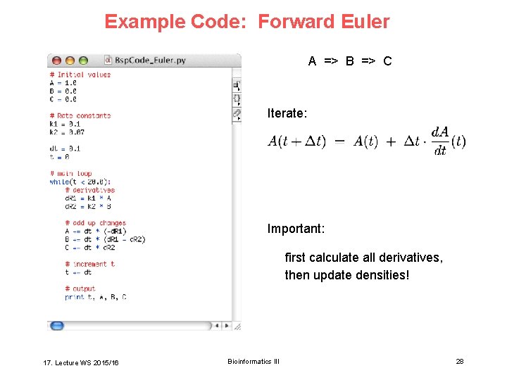
Example Code: Forward Euler A => B => C Iterate: Important: first calculate all derivatives, then update densities! 17. Lecture WS 2015/16 Bioinformatics III 28

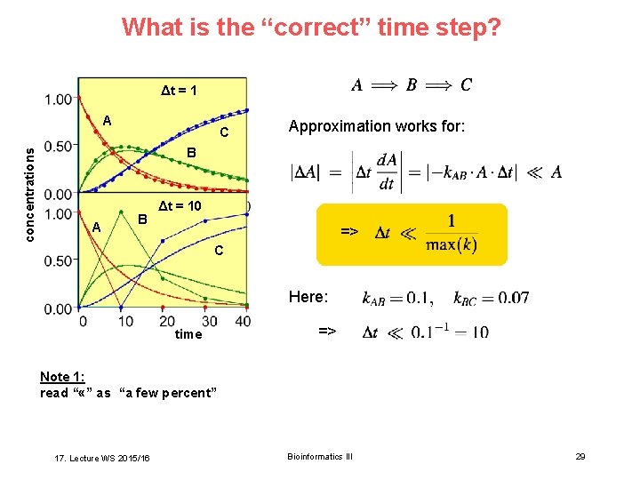
What is the “correct” time step? Δt = 1 concentrations A C Approximation works for: B A B Δt = 10 => C Here: time => Note 1: read “ «” as “a few percent” 17. Lecture WS 2015/16 Bioinformatics III 29

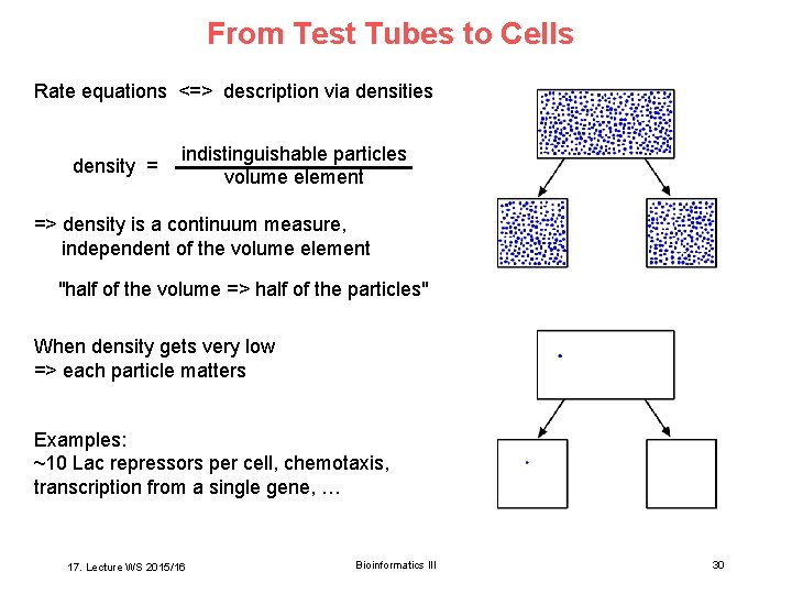
From Test Tubes to Cells Rate equations <=> description via densities density = indistinguishable particles volume element => density is a continuum measure, independent of the volume element "half of the volume => half of the particles" When density gets very low => each particle matters Examples: ~10 Lac repressors per cell, chemotaxis, transcription from a single gene, … 17. Lecture WS 2015/16 Bioinformatics III 30

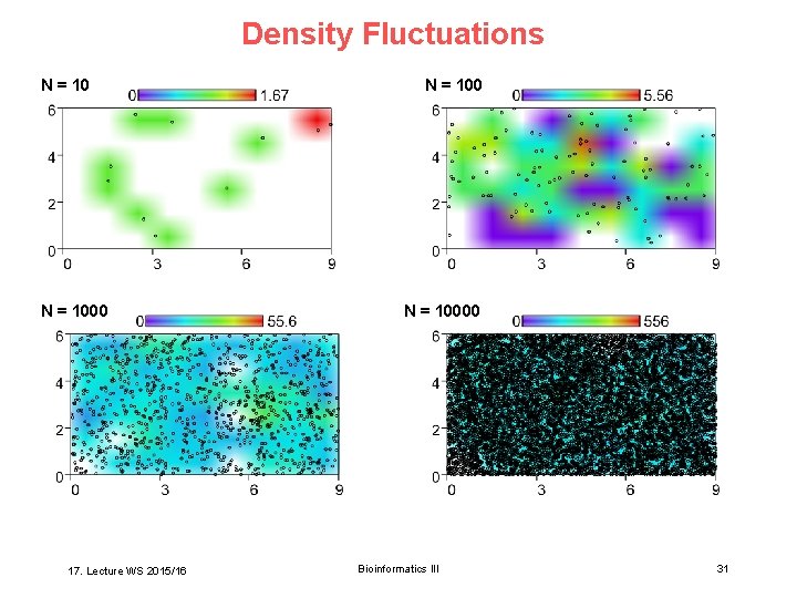
Density Fluctuations N = 1000 17. Lecture WS 2015/16 N = 10000 Bioinformatics III 31

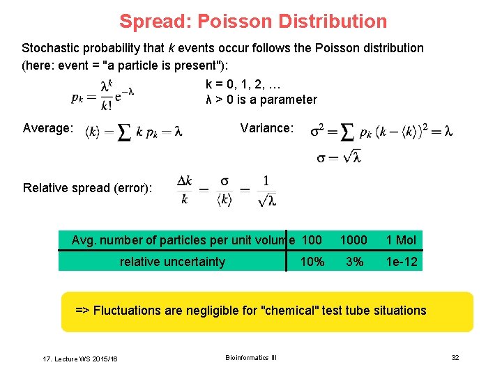
Spread: Poisson Distribution Stochastic probability that k events occur follows the Poisson distribution (here: event = "a particle is present"): k = 0, 1, 2, … λ > 0 is a parameter Average: Variance: Relative spread (error): Avg. number of particles per unit volume 100 relative uncertainty 10% 1000 1 Mol 3% 1 e-12 => Fluctuations are negligible for "chemical" test tube situations 17. Lecture WS 2015/16 Bioinformatics III 32

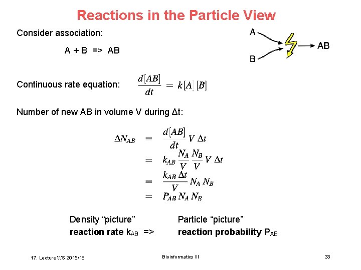
Reactions in the Particle View Consider association: A + B => AB Continuous rate equation: Number of new AB in volume V during Δt: Density “picture” reaction rate k. AB => 17. Lecture WS 2015/16 Particle “picture” reaction probability PAB Bioinformatics III 33

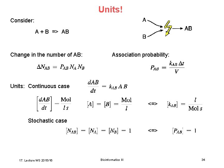
Units! Consider: A + B => AB Change in the number of AB: Association probability: Units: Continuous case <=> Stochastic case <=> 17. Lecture WS 2015/16 Bioinformatics III 34

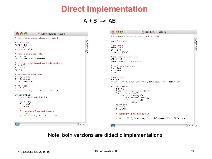
Direct Implementation A + B => AB Note: both versions are didactic implementations 17. Lecture WS 2015/16 Bioinformatics III 35

Example: Chained Reactions A => B => C Rates: NA, NB, NC [NA 0] Time course from continuous rate equations (benchmark): k 1 = k 2 = 0. 3 (units? ) 17. Lecture WS 2015/16 Bioinformatics III 36

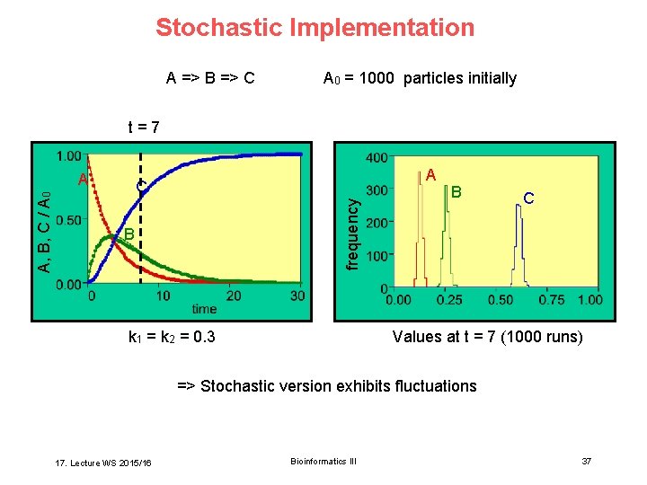
Stochastic Implementation A => B => C A 0 = 1000 particles initially t=7 A C frequency A, B, C / A 0 A B k 1 = k 2 = 0. 3 B C Values at t = 7 (1000 runs) => Stochastic version exhibits fluctuations 17. Lecture WS 2015/16 Bioinformatics III 37

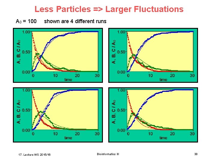
Less Particles => Larger Fluctuations A, B, C / A 0 17. Lecture WS 2015/16 A, B, C / A 0 shown are 4 different runs A, B, C / A 0 = 100 Bioinformatics III 38

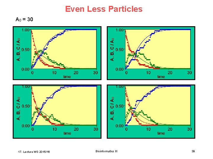
Even Less Particles 17. Lecture WS 2015/16 A, B, C / A 0 A 0 = 30 Bioinformatics III 39

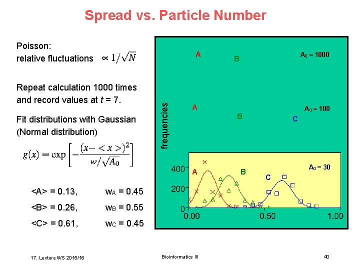
Spread vs. Particle Number Poisson: relative fluctuations Repeat calculation 1000 times and record values at t = 7. Fit distributions with Gaussian (Normal distribution) frequencies A A w. A = 0. 45 <B> = 0. 26, w. B = 0. 55 <C> = 0. 61, w. C = 0. 45 17. Lecture WS 2015/16 A 0 = 100 B A <A> = 0. 13, A 0 = 1000 B Bioinformatics III B C A 0 = 30 C 40

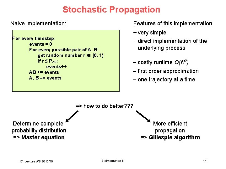
Stochastic Propagation Features of this implementation Naive implementation: + very simple For every timestep: events = 0 For every possible pair of A, B: get random number r ∈ [0, 1) if r ≤ PAB: events++ AB += events A, B –= events + direct implementation of the underlying process – costly runtime O(N 2) – first order approximation – one trajectory at a time => how to do better? ? ? More efficient propagation => Gillespie algorithm Determine complete probability distribution => Master equation 17. Lecture WS 2015/16 Bioinformatics III 41

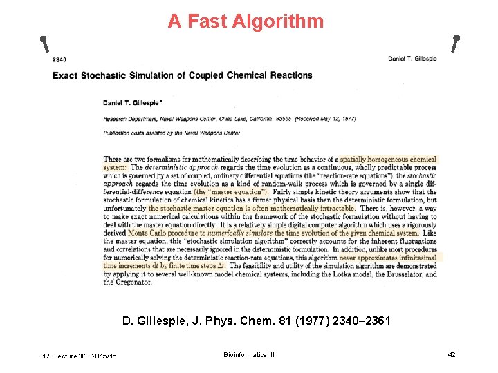
A Fast Algorithm D. Gillespie, J. Phys. Chem. 81 (1977) 2340– 2361 17. Lecture WS 2015/16 Bioinformatics III 42

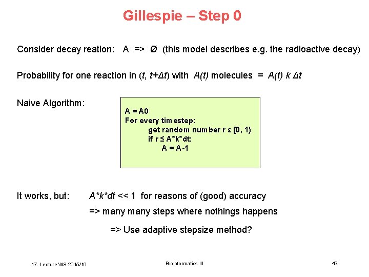
Gillespie – Step 0 Consider decay reation: A => Ø (this model describes e. g. the radioactive decay) Probability for one reaction in (t, t+Δt) with A(t) molecules = A(t) k Δt Naive Algorithm: It works, but: A = A 0 For every timestep: get random number r ε [0, 1) if r ≤ A*k*dt: A = A-1 A*k*dt << 1 for reasons of (good) accuracy => many steps where nothings happens => Use adaptive stepsize method? 17. Lecture WS 2015/16 Bioinformatics III 43

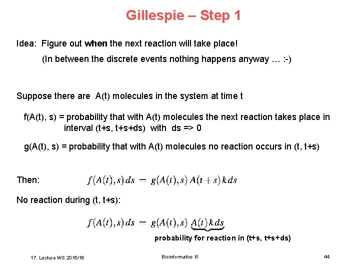
Gillespie – Step 1 Idea: Figure out when the next reaction will take place! (In between the discrete events nothing happens anyway … : -) Suppose there are A(t) molecules in the system at time t f(A(t), s) = probability that with A(t) molecules the next reaction takes place in interval (t+s, t+s+ds) with ds => 0 g(A(t), s) = probability that with A(t) molecules no reaction occurs in (t, t+s) Then: No reaction during (t, t+s): probability for reaction in (t+s, t+s+ds) 17. Lecture WS 2015/16 Bioinformatics III 44

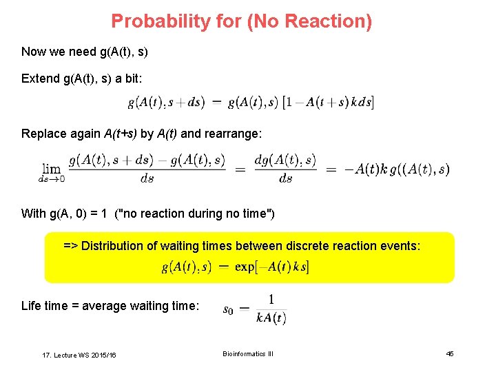
Probability for (No Reaction) Now we need g(A(t), s) Extend g(A(t), s) a bit: Replace again A(t+s) by A(t) and rearrange: With g(A, 0) = 1 ("no reaction during no time") => Distribution of waiting times between discrete reaction events: Life time = average waiting time: 17. Lecture WS 2015/16 Bioinformatics III 45

Exponentially Distributed Random Numbers Solve for s: r ε [0, 1] Exponential probability distribution: life time Simple Gillespie algorithm for the decay reaction A => Ø : A = A 0 While(A > 0): get random number r ε [0, 1) t = t + s(r) A=A-1 17. Lecture WS 2015/16 Bioinformatics III 46

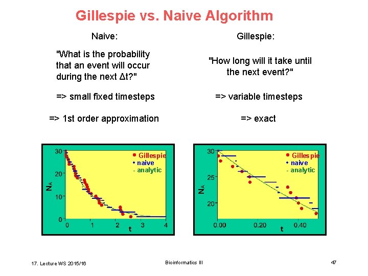
Gillespie vs. Naive Algorithm Naive: Gillespie: "What is the probability that an event will occur during the next Δt? " "How long will it take until the next event? " => small fixed timesteps => variable timesteps => 1 st order approximation => exact • Gillespie • naive - analytic NA NA • naive - analytic t 17. Lecture WS 2015/16 t Bioinformatics III 47

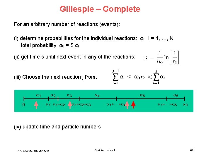
Gillespie – Complete For an arbitrary number of reactions (events): (i) determine probabilities for the individual reactions: αi i = 1, …, N total probability α 0 = Σ αi (ii) get time s until next event in any of the reactions: (iii) Choose the next reaction j from: (iv) update time and particle numbers 17. Lecture WS 2015/16 Bioinformatics III 48

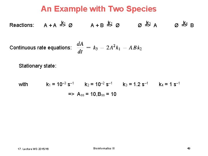
An Example with Two Species Reactions: k 1 Ø A + A => k 2 Ø A + B => k 3 A Ø => k 4 B Ø => Continuous rate equations: Stationary state: with k 1 = 10– 3 s– 1 k 2 = 10– 2 s– 1 k 3 = 1. 2 s– 1 k 4 = 1 s– 1 => Ass = 10, Bss = 10 17. Lecture WS 2015/16 Bioinformatics III 49

Erban, Chapman, Maini, ar. Xiv: 0704. 1908 v 2 [q-bio. SC] Gillespie Algorithm 17. Lecture WS 2015/16 Bioinformatics III 50

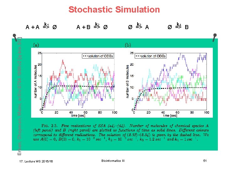
Stochastic Simulation k 1 k 2 A + B => Ø k 3 Ø => A k 4 Ø => B Erban, Chapman, Maini, ar. Xiv: 0704. 1908 v 2 [q-bio. SC] A + A => Ø 17. Lecture WS 2015/16 Bioinformatics III 51

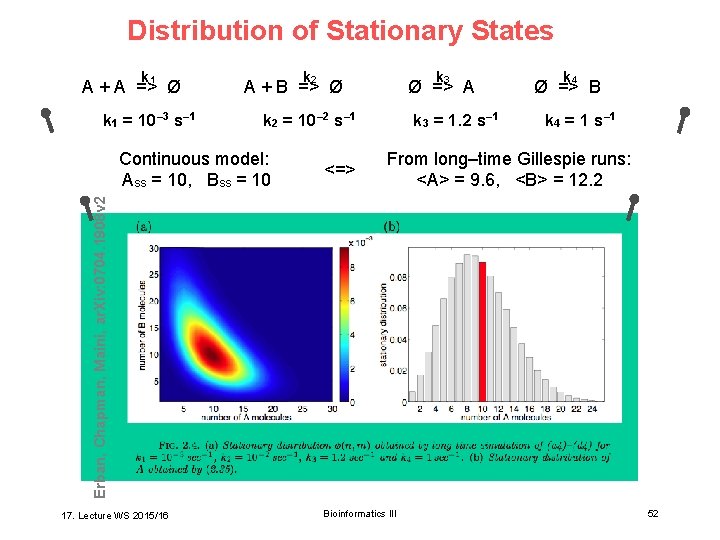
Distribution of Stationary States k 1 A + A => Ø k 1 = 10– 3 s– 1 k 2 k 3 A + B => Ø Ø => A k 2 = 10– 2 s– 1 <=> k 4 = 1 s– 1 From long–time Gillespie runs: <A> = 9. 6, <B> = 12. 2 Erban, Chapman, Maini, ar. Xiv: 0704. 1908 v 2 Continuous model: Ass = 10, Bss = 10 k 3 = 1. 2 s– 1 k 4 Ø => B 17. Lecture WS 2015/16 Bioinformatics III 52

Stochastic vs. Continuous For many simple systems: stochastic solution looks like noisy deterministic solution Yet in some cases, stochastic description gives qualitatively different results • swapping between two stationary states • noise-induced oscillations • Lotka-Volterra with small populations • sensitivity in signalling 17. Lecture WS 2015/16 Bioinformatics III 53

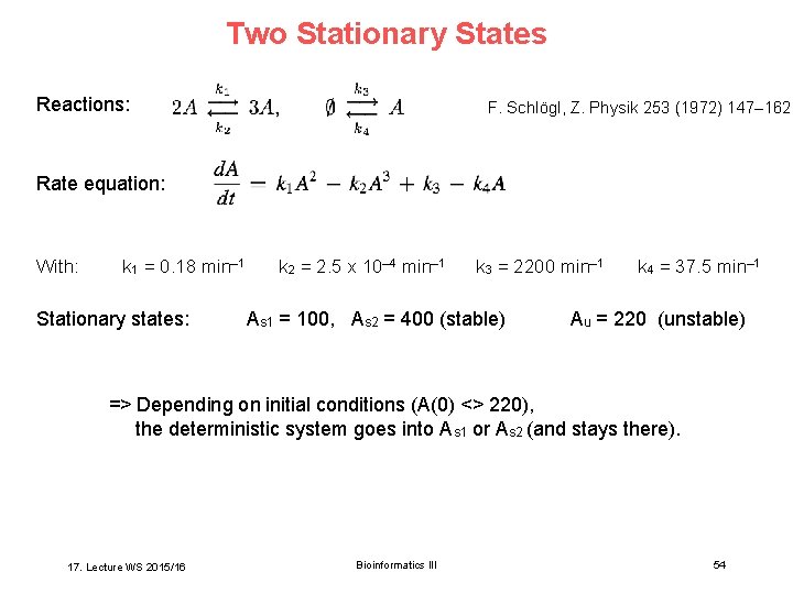
Two Stationary States Reactions: F. Schlögl, Z. Physik 253 (1972) 147– 162 Rate equation: With: k 1 = 0. 18 min– 1 Stationary states: k 2 = 2. 5 x 10– 4 min– 1 k 3 = 2200 min– 1 As 1 = 100, As 2 = 400 (stable) k 4 = 37. 5 min– 1 Au = 220 (unstable) => Depending on initial conditions (A(0) <> 220), the deterministic system goes into As 1 or As 2 (and stays there). 17. Lecture WS 2015/16 Bioinformatics III 54

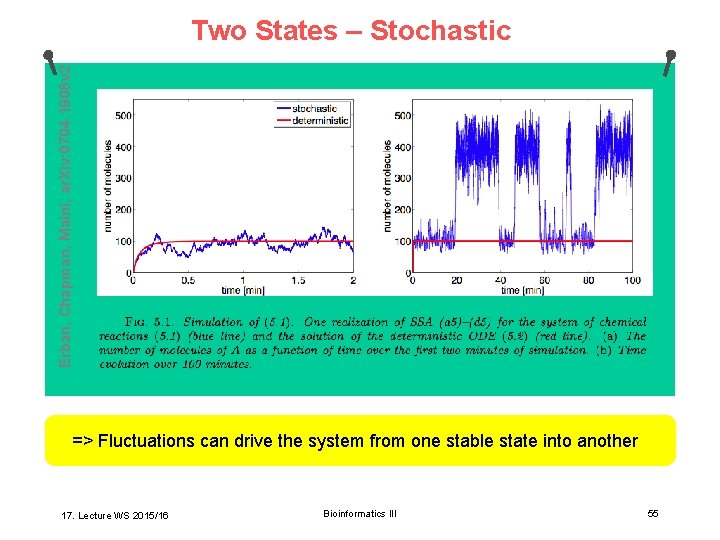
Erban, Chapman, Maini, ar. Xiv: 0704. 1908 v 2 Two States – Stochastic => Fluctuations can drive the system from one stable state into another 17. Lecture WS 2015/16 Bioinformatics III 55

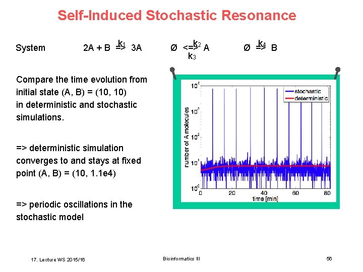
Self-Induced Stochastic Resonance System k 2 A + B =>1 3 A k Ø <=>2 A k 3 k Ø =>4 B Compare the time evolution from initial state (A, B) = (10, 10) in deterministic and stochastic simulations. => deterministic simulation converges to and stays at fixed point (A, B) = (10, 1. 1 e 4) => periodic oscillations in the stochastic model 17. Lecture WS 2015/16 Bioinformatics III 56

Summary • Mass action kinetics => solving (integrating) differential equations for time-dependent behavior => Forward-Euler: extrapolation, time steps • Stochastic Description => why stochastic? => Gillespie algorithm => different dynamic behavior 17. Lecture WS 2015/16 Bioinformatics III 57