V 1 Introduction A cell is a crowded

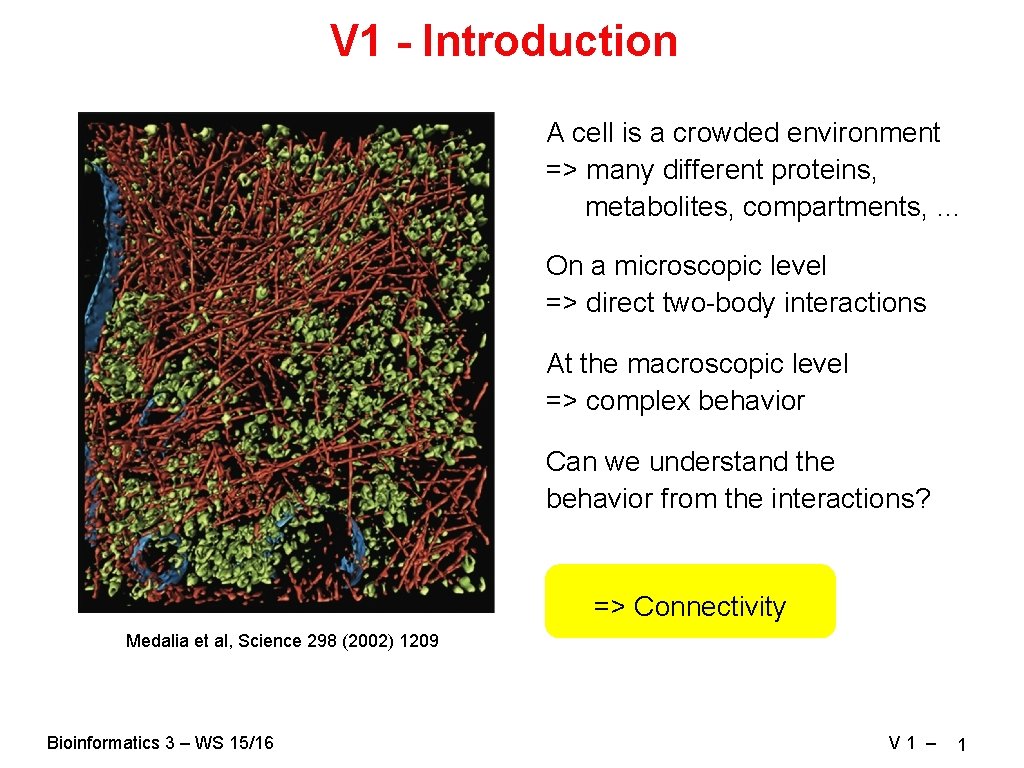
V 1 - Introduction A cell is a crowded environment => many different proteins, metabolites, compartments, … On a microscopic level => direct two-body interactions At the macroscopic level => complex behavior Can we understand the behavior from the interactions? => Connectivity Medalia et al, Science 298 (2002) 1209 Bioinformatics 3 – WS 15/16 V 1 – 1

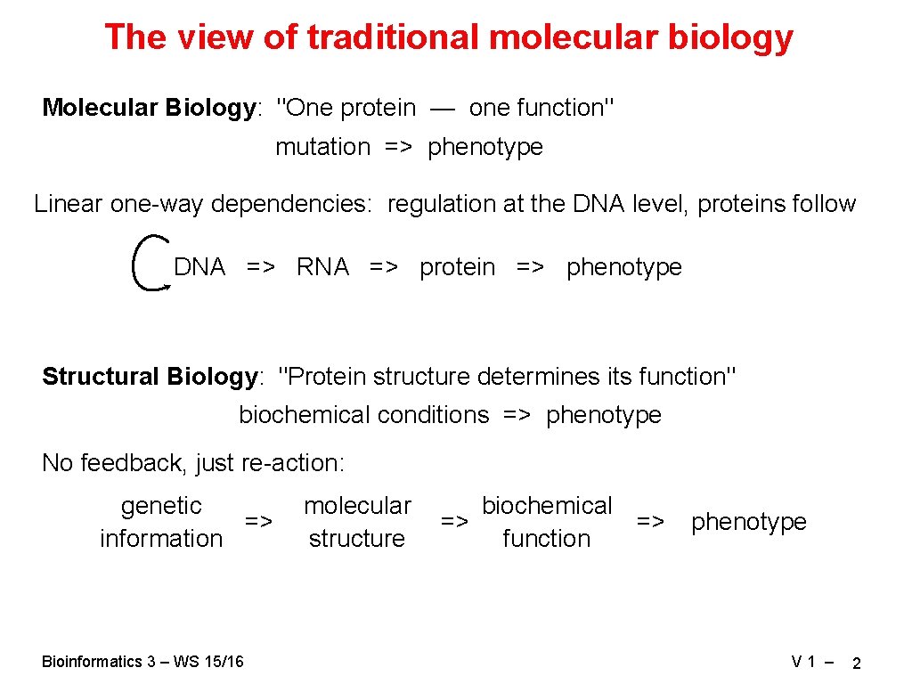
The view of traditional molecular biology Molecular Biology: "One protein — one function" mutation => phenotype Linear one-way dependencies: regulation at the DNA level, proteins follow DNA => RNA => protein => phenotype Structural Biology: "Protein structure determines its function" biochemical conditions => phenotype No feedback, just re-action: genetic => information Bioinformatics 3 – WS 15/16 molecular biochemical => => structure function phenotype V 1 – 2

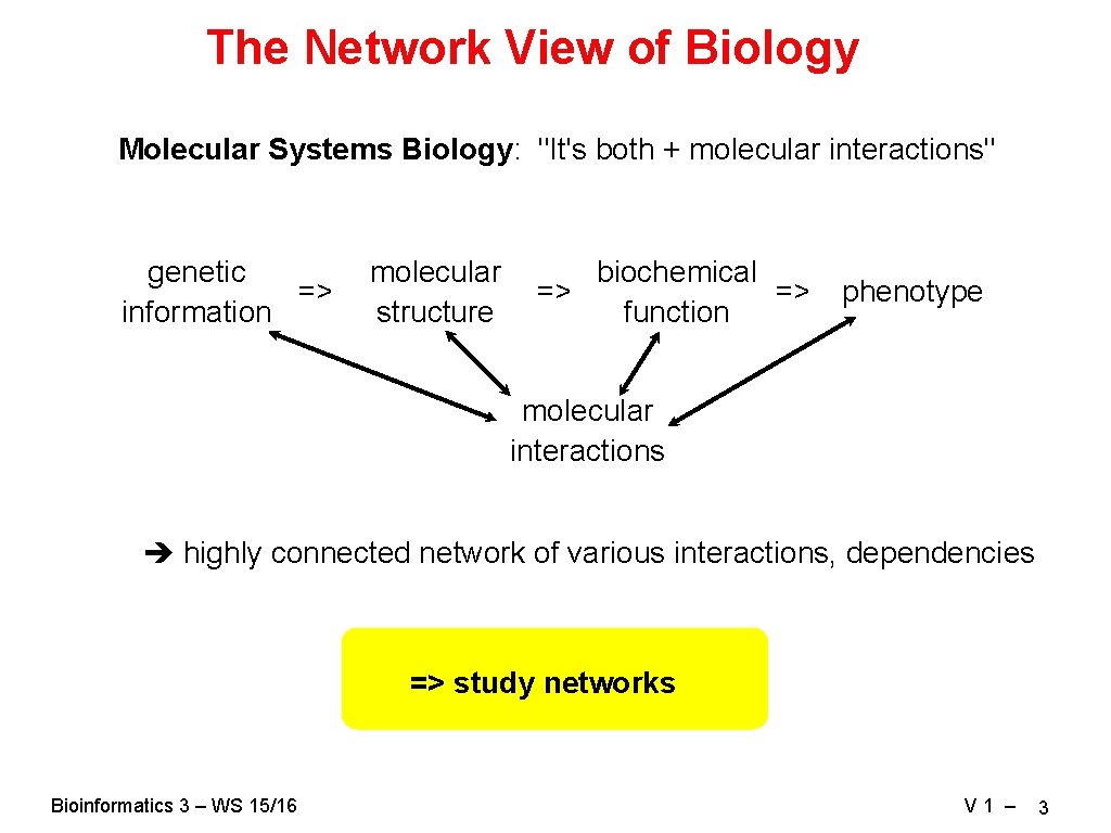
The Network View of Biology Molecular Systems Biology: "It's both + molecular interactions" genetic => information molecular biochemical => => structure function phenotype molecular interactions highly connected network of various interactions, dependencies => study networks Bioinformatics 3 – WS 15/16 V 1 – 3

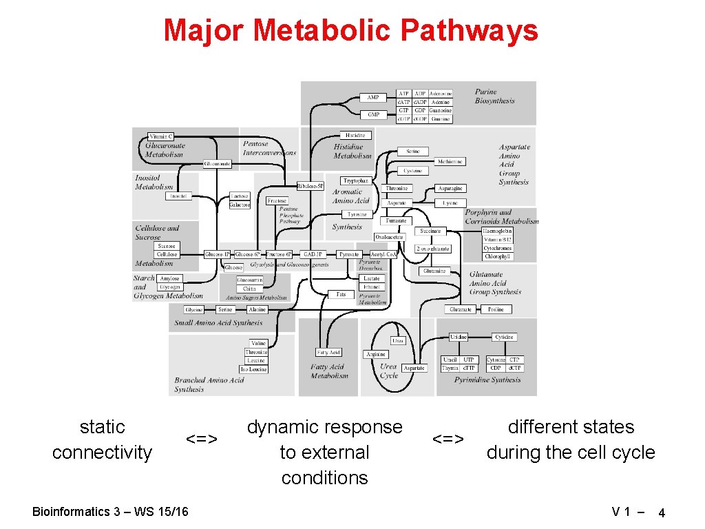
Major Metabolic Pathways static connectivity <=> Bioinformatics 3 – WS 15/16 dynamic response to external conditions <=> different states during the cell cycle V 1 – 4

Bioinformatics 3 – WS 15/16 http: //www. mvv-muenchen. de/de/netzbahnhoefe/netzplaene/index. html V 1 – 5

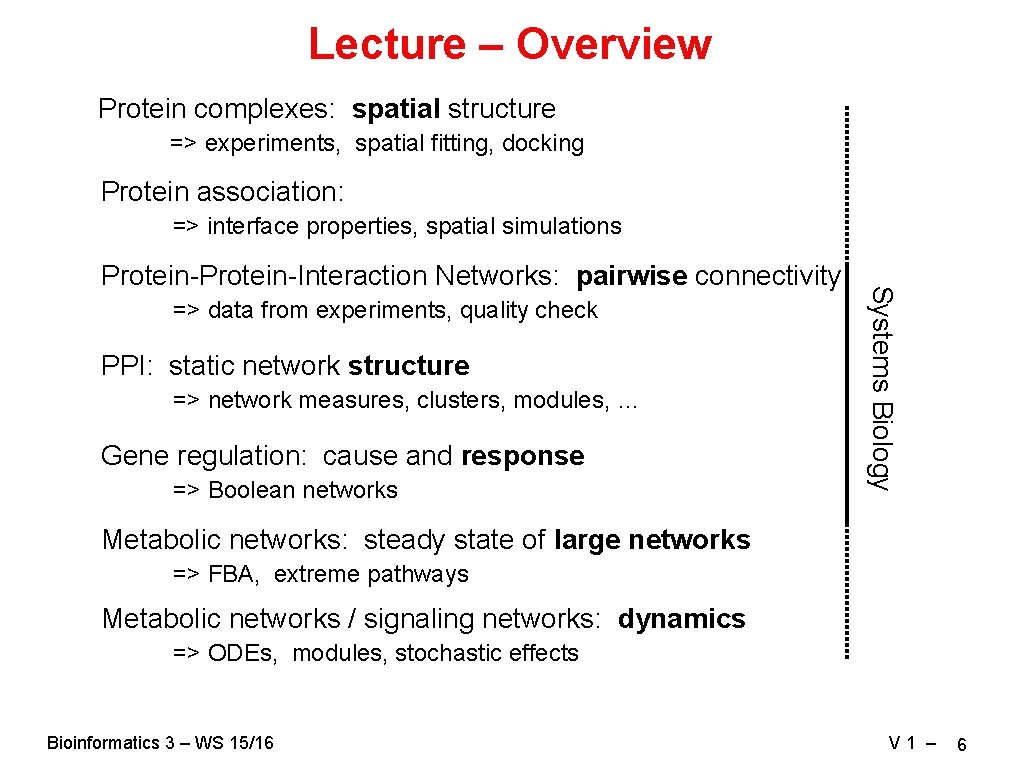
Lecture – Overview Protein complexes: spatial structure => experiments, spatial fitting, docking Protein association: => interface properties, spatial simulations => data from experiments, quality check PPI: static network structure => network measures, clusters, modules, … Gene regulation: cause and response => Boolean networks Systems Biology Protein-Interaction Networks: pairwise connectivity Metabolic networks: steady state of large networks => FBA, extreme pathways Metabolic networks / signaling networks: dynamics => ODEs, modules, stochastic effects Bioinformatics 3 – WS 15/16 V 1 – 6

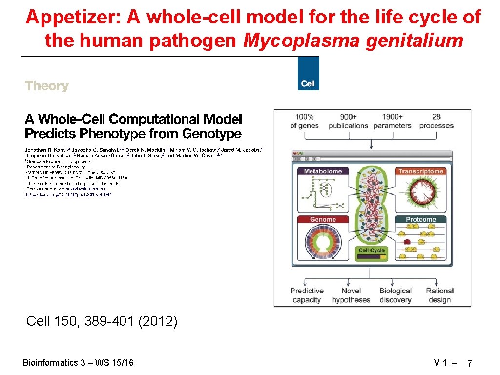
Appetizer: A whole-cell model for the life cycle of the human pathogen Mycoplasma genitalium Cell 150, 389 -401 (2012) Bioinformatics 3 – WS 15/16 V 1 – 7

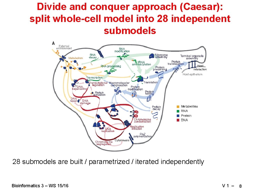
Divide and conquer approach (Caesar): split whole-cell model into 28 independent submodels 28 submodels are built / parametrized / iterated independently Bioinformatics 3 – WS 15/16 V 1 – 8

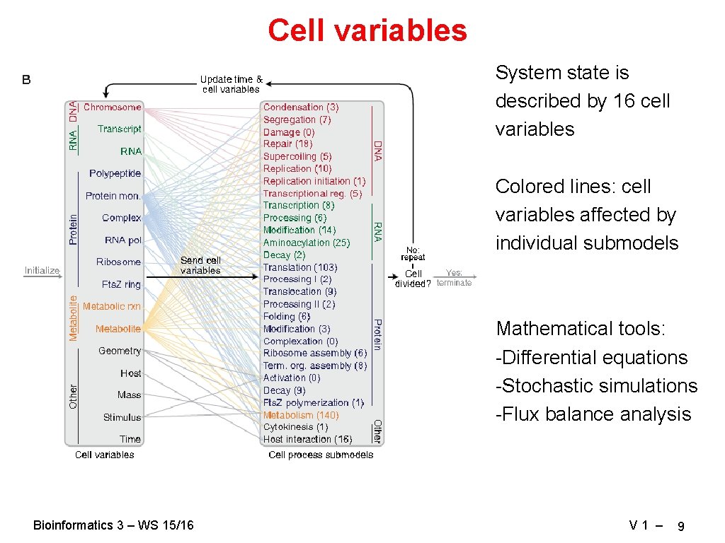
Cell variables System state is described by 16 cell variables Colored lines: cell variables affected by individual submodels Mathematical tools: -Differential equations -Stochastic simulations -Flux balance analysis Bioinformatics 3 – WS 15/16 V 1 – 9

Bioinformatics 3 – WS 15/16 V 1 – 10

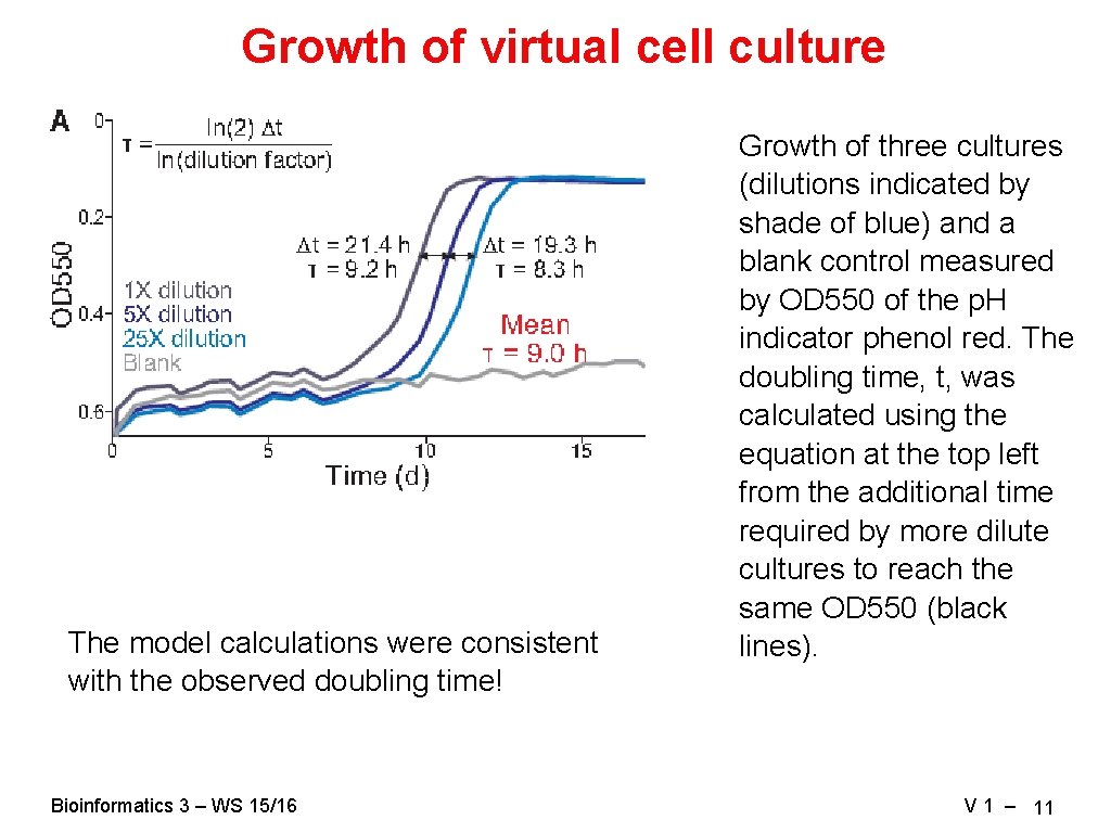
Growth of virtual cell culture The model calculations were consistent with the observed doubling time! Bioinformatics 3 – WS 15/16 Growth of three cultures (dilutions indicated by shade of blue) and a blank control measured by OD 550 of the p. H indicator phenol red. The doubling time, t, was calculated using the equation at the top left from the additional time required by more dilute cultures to reach the same OD 550 (black lines). V 1 – 11

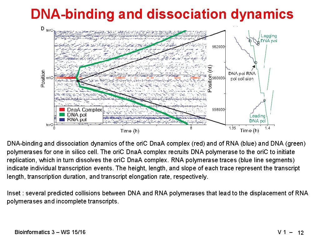
DNA-binding and dissociation dynamics of the ori. C Dna. A complex (red) and of RNA (blue) and DNA (green) polymerases for one in silico cell. The ori. C Dna. A complex recruits DNA polymerase to the ori. C to initiate replication, which in turn dissolves the ori. C Dna. A complex. RNA polymerase traces (blue line segments) indicate individual transcription events. The height, length, and slope of each trace represent the transcript length, transcription duration, and transcript elongation rate, respectively. Inset : several predicted collisions between DNA and RNA polymerases that lead to the displacement of RNA polymerases and incomplete transcripts. Bioinformatics 3 – WS 15/16 V 1 – 12

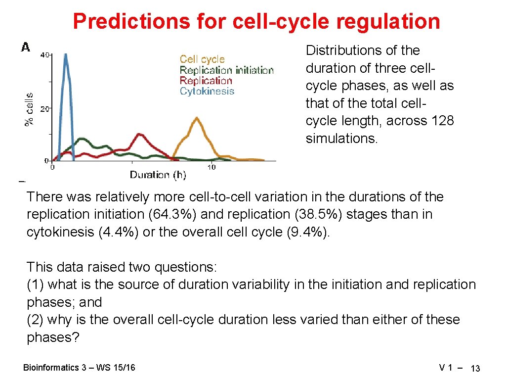
Predictions for cell-cycle regulation Distributions of the duration of three cellcycle phases, as well as that of the total cellcycle length, across 128 simulations. There was relatively more cell-to-cell variation in the durations of the replication initiation (64. 3%) and replication (38. 5%) stages than in cytokinesis (4. 4%) or the overall cell cycle (9. 4%). This data raised two questions: (1) what is the source of duration variability in the initiation and replication phases; and (2) why is the overall cell-cycle duration less varied than either of these phases? Bioinformatics 3 – WS 15/16 V 1 – 13

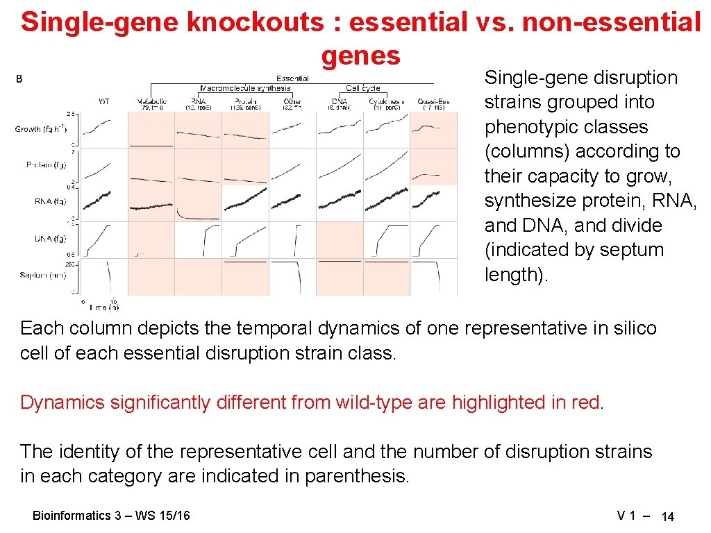
Single-gene knockouts : essential vs. non-essential genes Single-gene disruption strains grouped into phenotypic classes (columns) according to their capacity to grow, synthesize protein, RNA, and DNA, and divide (indicated by septum length). Each column depicts the temporal dynamics of one representative in silico cell of each essential disruption strain class. Dynamics significantly different from wild-type are highlighted in red. The identity of the representative cell and the number of disruption strains in each category are indicated in parenthesis. Bioinformatics 3 – WS 15/16 V 1 – 14

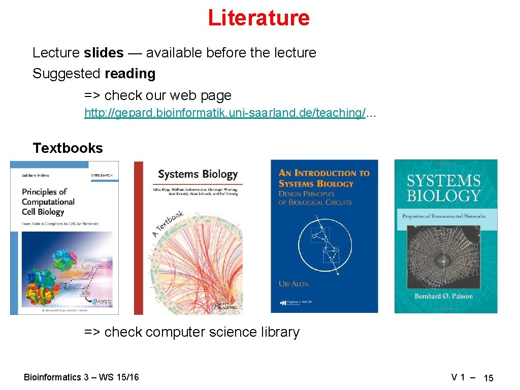
Literature Lecture slides — available before the lecture Suggested reading => check our web page http: //gepard. bioinformatik. uni-saarland. de/teaching/… Textbooks => check computer science library Bioinformatics 3 – WS 15/16 V 1 – 15

How to pass this course Schein = you need to qualify for the final exam and pass it Final exam: written test of 180 min length about selected parts of the lecture (will be defined 2 weeks before exam) and about the assignments requirements for participation: • 50% of the points from the assignments • one assignment task presented @ blackboard Final exam will take place at the end of the semester In case you are sick (final exam) you should bring a medical certificate to get a re-exam. Re-exam: will take place in first week of the summer term 2016 Bioinformatics 3 – WS 15/16 V 1 – 16

Assignments Tutors: Thorsten Will, Maryam Nazarieh Duy Nguyen, Ha Vu Tranh Tutorial: ? ? Mon, 12: 00– 14: 00, E 2 1, room 007 10 assignments with 100 points each Assignments are part of the course material (not everything is covered in lecture) => one solution for two students (or one) => hand-written or one printable PDF/PS file per email => content: data analysis + interpretation — think! => no 100% solutions required!!! => attach the source code of the programs for checking (no suppl. data) => present one task at the blackboard Hand in at the following Fri electronically until 13: 00 or printed at the start of the lecture. Bioinformatics 3 – WS 15/16 V 1 – 17

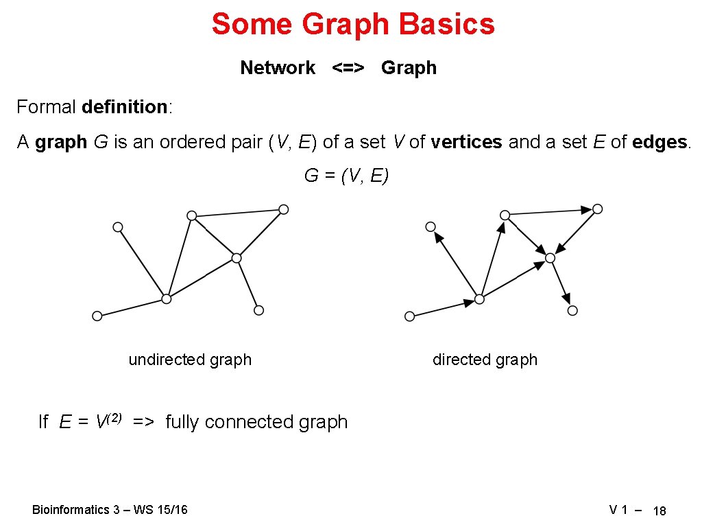
Some Graph Basics Network <=> Graph Formal definition: A graph G is an ordered pair (V, E) of a set V of vertices and a set E of edges. G = (V, E) undirected graph If E = V(2) => fully connected graph Bioinformatics 3 – WS 15/16 V 1 – 18

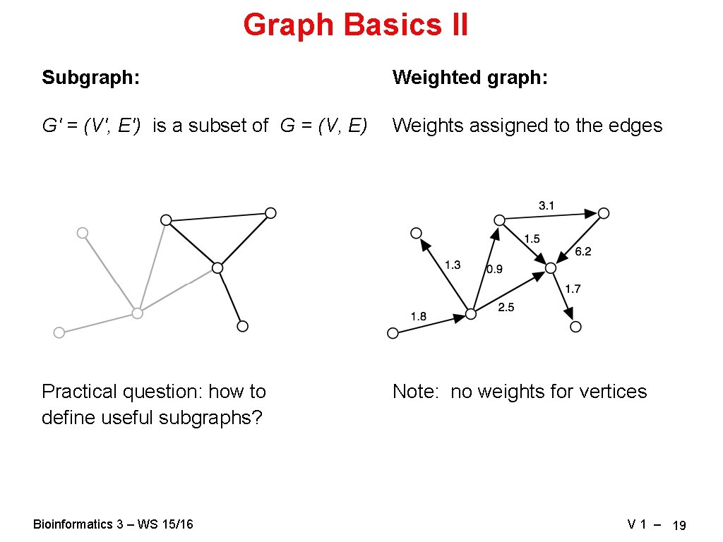
Graph Basics II Subgraph: Weighted graph: G' = (V', E') is a subset of G = (V, E) Weights assigned to the edges Practical question: how to define useful subgraphs? Note: no weights for vertices Bioinformatics 3 – WS 15/16 V 1 – 19

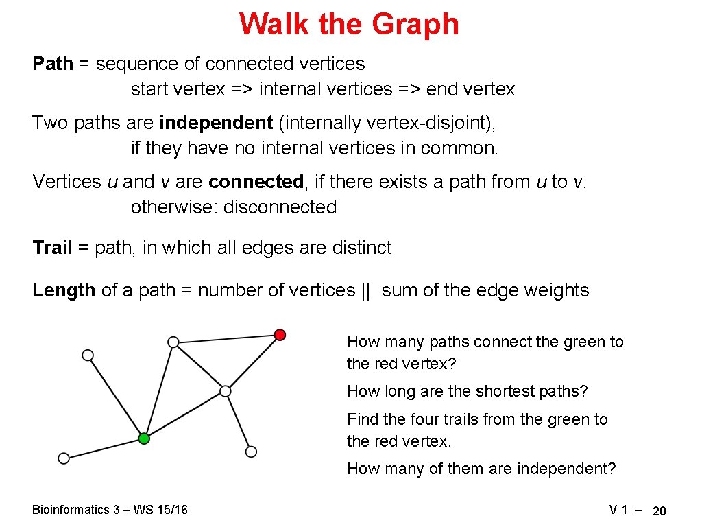
Walk the Graph Path = sequence of connected vertices start vertex => internal vertices => end vertex Two paths are independent (internally vertex-disjoint), if they have no internal vertices in common. Vertices u and v are connected, if there exists a path from u to v. otherwise: disconnected Trail = path, in which all edges are distinct Length of a path = number of vertices || sum of the edge weights How many paths connect the green to the red vertex? How long are the shortest paths? Find the four trails from the green to the red vertex. How many of them are independent? Bioinformatics 3 – WS 15/16 V 1 – 20

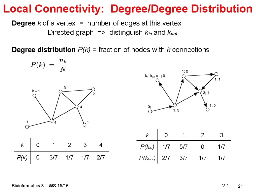
Local Connectivity: Degree/Degree Distribution Degree k of a vertex = number of edges at this vertex Directed graph => distinguish kin and kout Degree distribution P(k) = fraction of nodes with k connections k 0 1 2 3 4 P(kin) 1/7 5/7 0 1/7 P(k) 0 3/7 1/7 2/7 P(kout) 2/7 3/7 1/7 Bioinformatics 3 – WS 15/16 V 1 – 21

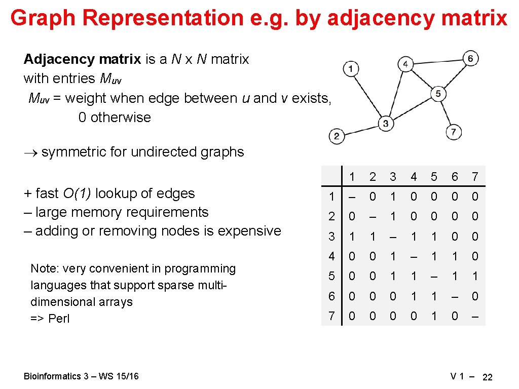
Graph Representation e. g. by adjacency matrix Adjacency matrix is a N x N matrix with entries Muv = weight when edge between u and v exists, 0 otherwise symmetric for undirected graphs + fast O(1) lookup of edges – large memory requirements – adding or removing nodes is expensive Note: very convenient in programming languages that support sparse multidimensional arrays => Perl Bioinformatics 3 – WS 15/16 1 2 3 4 5 6 7 1 – 0 1 0 0 2 0 – 1 0 0 3 1 1 – 1 1 0 0 4 0 0 1 – 1 1 0 5 0 0 1 1 – 1 1 6 0 0 0 1 1 – 0 7 0 0 1 0 – V 1 – 22

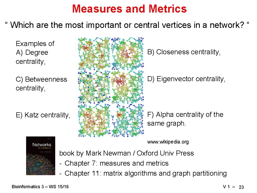
Measures and Metrics “ Which are the most important or central vertices in a network? “ Examples of A) Degree centrality, B) Closeness centrality, C) Betweenness centrality, D) Eigenvector centrality, E) Katz centrality, F) Alpha centrality of the same graph. www. wikipedia. org book by Mark Newman / Oxford Univ Press - Chapter 7: measures and metrics - Chapter 11: matrix algorithms and graph partitioning Bioinformatics 3 – WS 15/16 V 1 – 23

Degree centrality Perhaps the simplest centrality measure in a network is the degree centrality that is simply equal to the degree of each vertex. E. g. in a social network, individuals that have many connections to others might have - more influence, - more access to information, - or more prestige than those individuals who have fewer connections. A natural extension of the simple degree centrality is eigenvector centrality. Bioinformatics 3 – WS 15/16 V 1 – 24

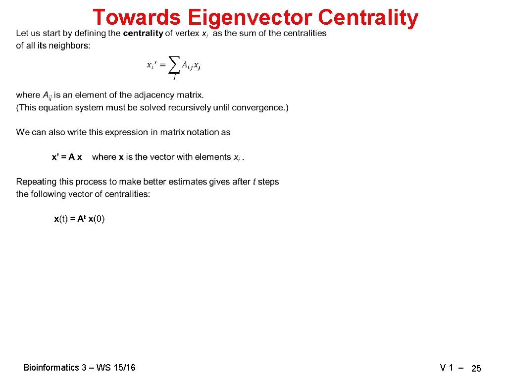
Towards Eigenvector Centrality Bioinformatics 3 – WS 15/16 V 1 – 25

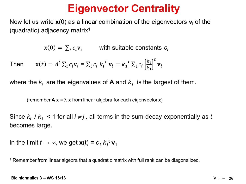
Eigenvector Centrality Bioinformatics 3 – WS 15/16 V 1 – 26

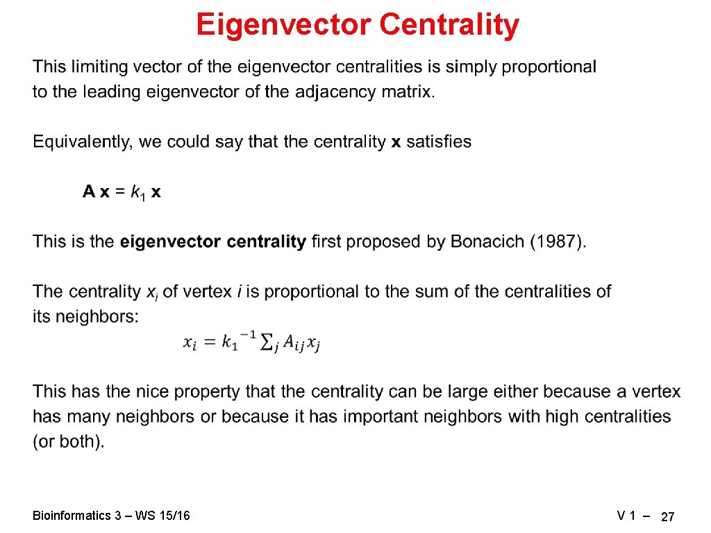
Eigenvector Centrality Bioinformatics 3 – WS 15/16 V 1 – 27

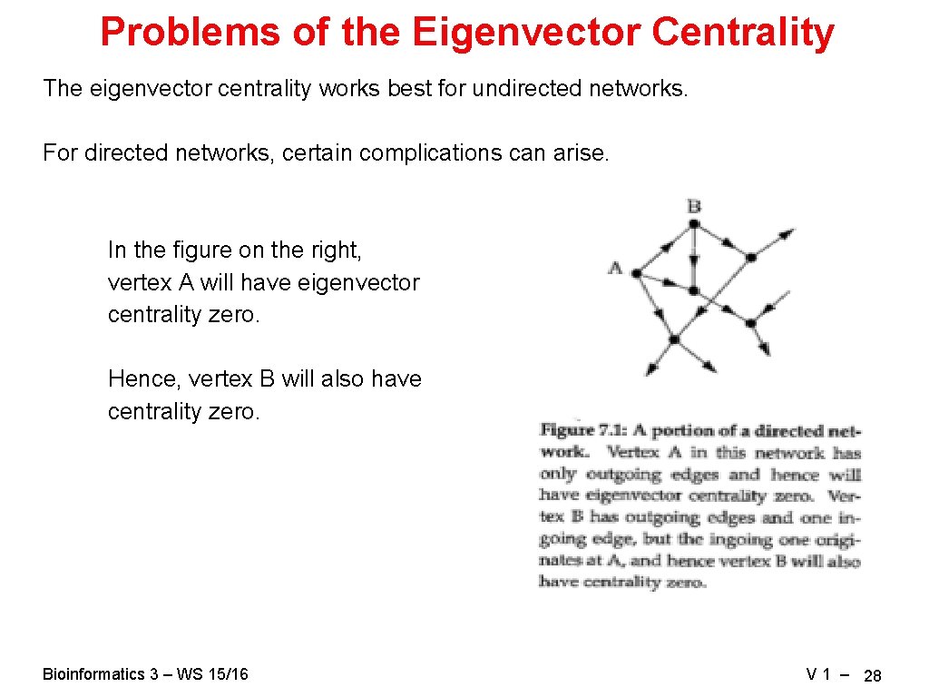
Problems of the Eigenvector Centrality The eigenvector centrality works best for undirected networks. For directed networks, certain complications can arise. In the figure on the right, vertex A will have eigenvector centrality zero. Hence, vertex B will also have centrality zero. Bioinformatics 3 – WS 15/16 V 1 – 28

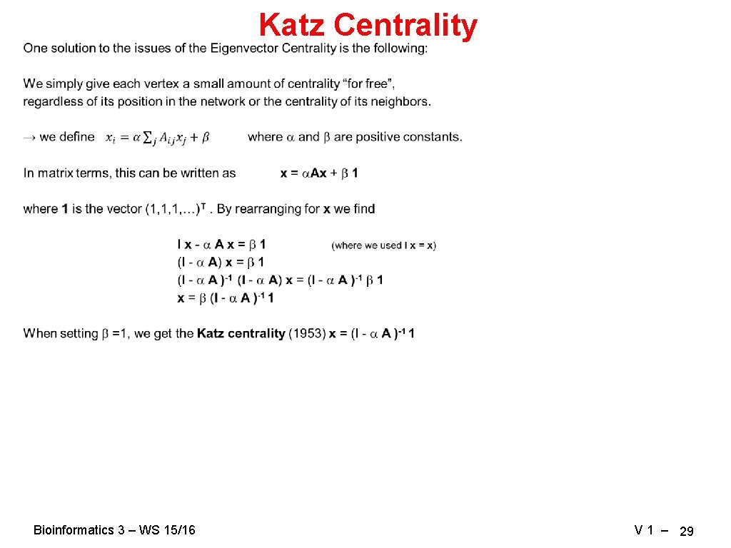
Katz Centrality Bioinformatics 3 – WS 15/16 V 1 – 29

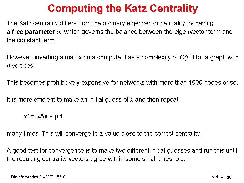
Computing the Katz Centrality The Katz centrality differs from the ordinary eigenvector centrality by having a free parameter , which governs the balance between the eigenvector term and the constant term. However, inverting a matrix on a computer has a complexity of O(n 3) for a graph with n vertices. This becomes prohibitively expensive for networks with more than 1000 nodes or so. It is more efficient to make an initial guess of x and then repeat x' = Ax + 1 many times. This will converge to a value close to the correct centrality. A good test for convergence is to make two different initial guesses and run this until the resulting centrality vectors agree within some small threshold. Bioinformatics 3 – WS 15/16 V 1 – 30

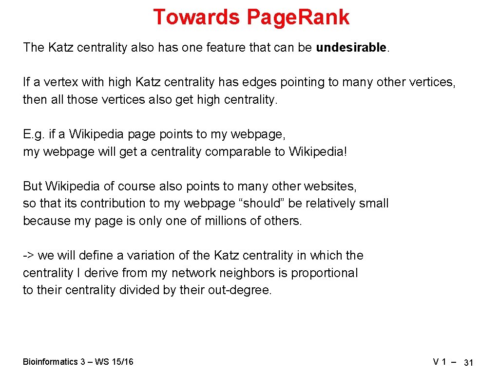
Towards Page. Rank The Katz centrality also has one feature that can be undesirable. If a vertex with high Katz centrality has edges pointing to many other vertices, then all those vertices also get high centrality. E. g. if a Wikipedia page points to my webpage, my webpage will get a centrality comparable to Wikipedia! But Wikipedia of course also points to many other websites, so that its contribution to my webpage “should” be relatively small because my page is only one of millions of others. -> we will define a variation of the Katz centrality in which the centrality I derive from my network neighbors is proportional to their centrality divided by their out-degree. Bioinformatics 3 – WS 15/16 V 1 – 31

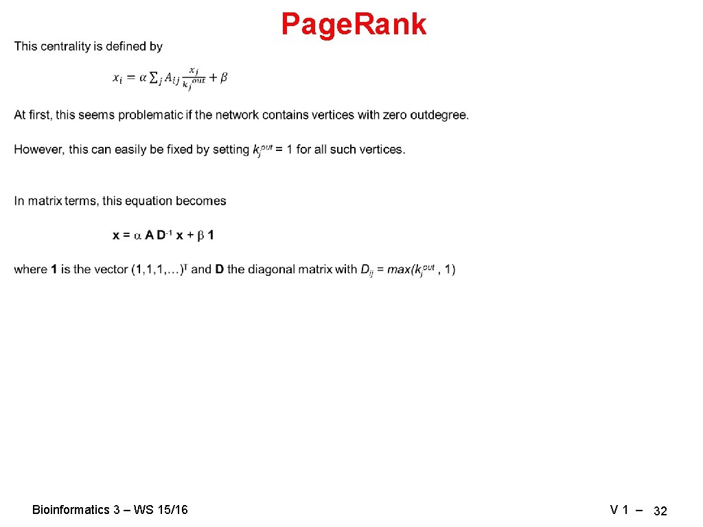
Page. Rank Bioinformatics 3 – WS 15/16 V 1 – 32

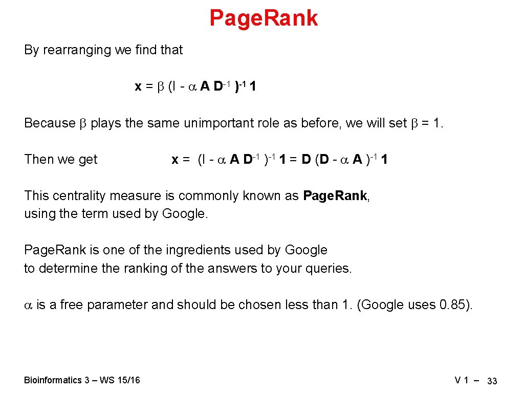
Page. Rank By rearranging we find that x = (I - A D-1 )-1 1 Because plays the same unimportant role as before, we will set = 1. Then we get x = (I - A D-1 )-1 1 = D (D - A )-1 1 This centrality measure is commonly known as Page. Rank, using the term used by Google. Page. Rank is one of the ingredients used by Google to determine the ranking of the answers to your queries. is a free parameter and should be chosen less than 1. (Google uses 0. 85). Bioinformatics 3 – WS 15/16 V 1 – 33

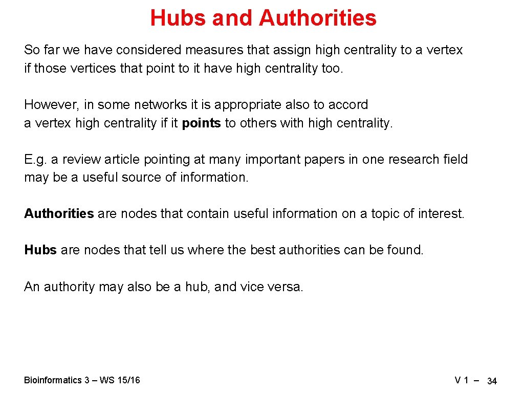
Hubs and Authorities So far we have considered measures that assign high centrality to a vertex if those vertices that point to it have high centrality too. However, in some networks it is appropriate also to accord a vertex high centrality if it points to others with high centrality. E. g. a review article pointing at many important papers in one research field may be a useful source of information. Authorities are nodes that contain useful information on a topic of interest. Hubs are nodes that tell us where the best authorities can be found. An authority may also be a hub, and vice versa. Bioinformatics 3 – WS 15/16 V 1 – 34

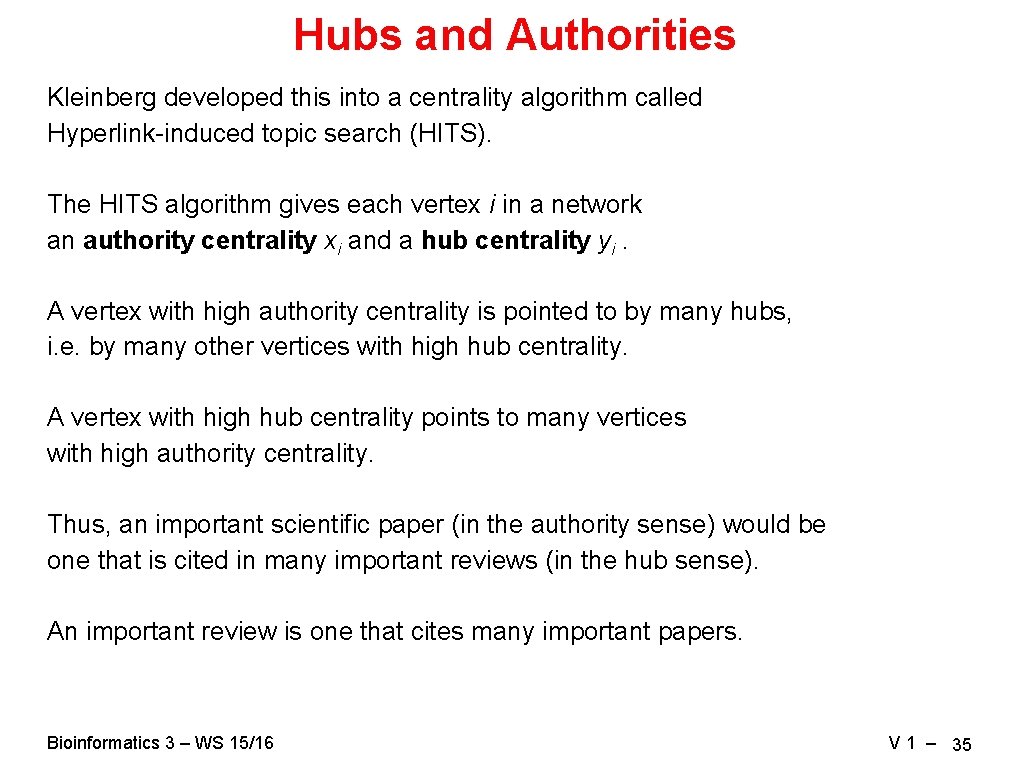
Hubs and Authorities Kleinberg developed this into a centrality algorithm called Hyperlink-induced topic search (HITS). The HITS algorithm gives each vertex i in a network an authority centrality xi and a hub centrality yi. A vertex with high authority centrality is pointed to by many hubs, i. e. by many other vertices with high hub centrality. A vertex with high hub centrality points to many vertices with high authority centrality. Thus, an important scientific paper (in the authority sense) would be one that is cited in many important reviews (in the hub sense). An important review is one that cites many important papers. Bioinformatics 3 – WS 15/16 V 1 – 35

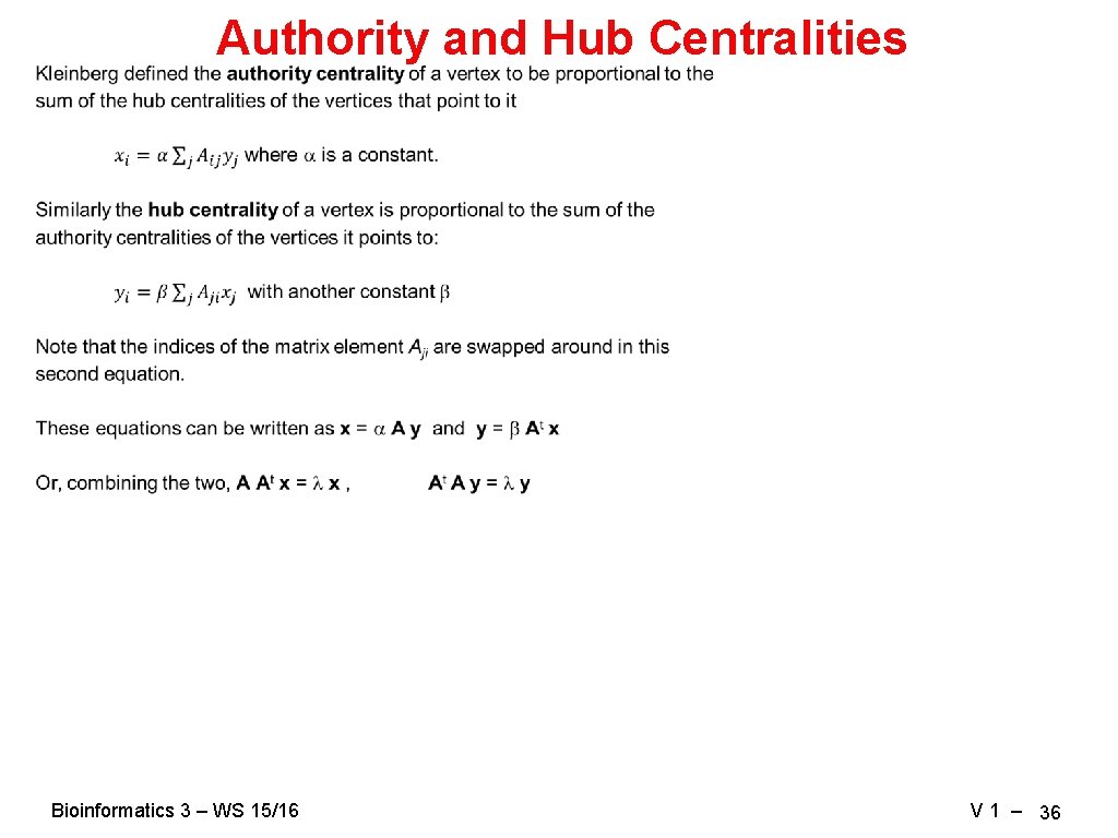
Authority and Hub Centralities Bioinformatics 3 – WS 15/16 V 1 – 36

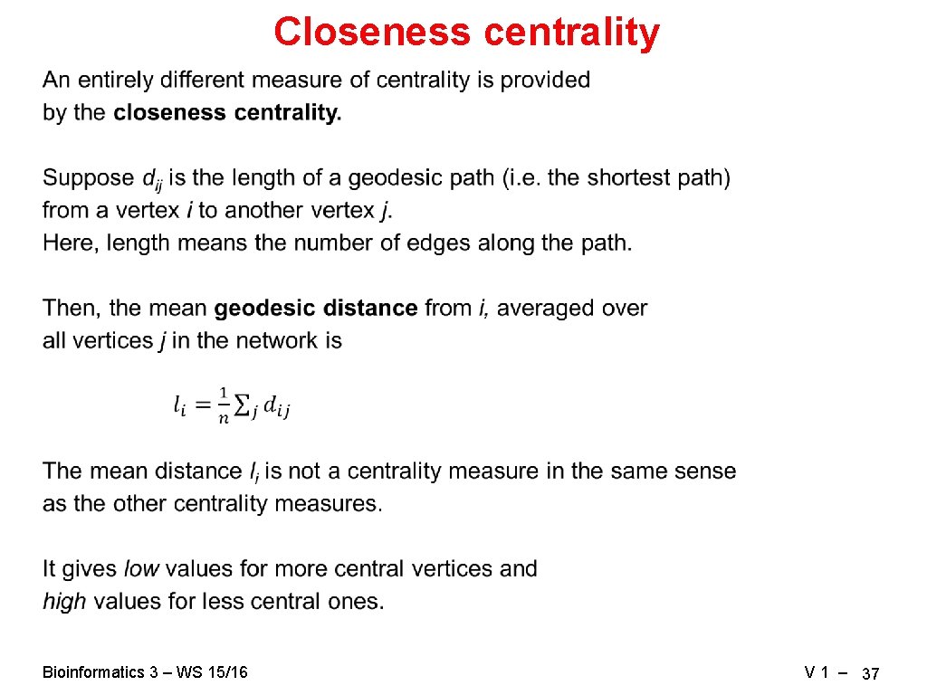
Closeness centrality Bioinformatics 3 – WS 15/16 V 1 – 37

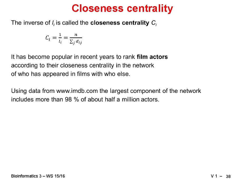
Closeness centrality Bioinformatics 3 – WS 15/16 V 1 – 38

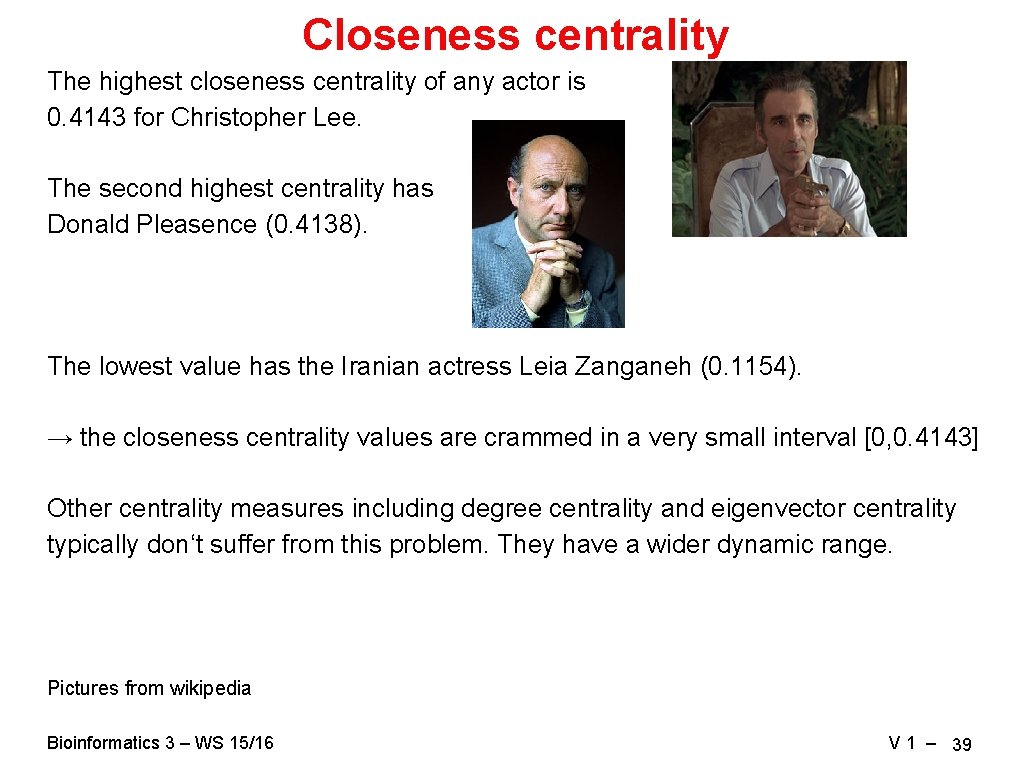
Closeness centrality The highest closeness centrality of any actor is 0. 4143 for Christopher Lee. The second highest centrality has Donald Pleasence (0. 4138). The lowest value has the Iranian actress Leia Zanganeh (0. 1154). → the closeness centrality values are crammed in a very small interval [0, 0. 4143] Other centrality measures including degree centrality and eigenvector centrality typically don‘t suffer from this problem. They have a wider dynamic range. Pictures from wikipedia Bioinformatics 3 – WS 15/16 V 1 – 39

Summary What you learned today: => networks are everywhere Þ how to get the "Schein" for BI 3 Þ How to determine the most central nodes in a network Next lecture: => basic network types and definitions: random, scale-free, degree distribution, Poisson distribution, ageing, … => clusters, percolation => algorithm on a graph: Dijkstra's shortest path algorithm => looking at graphs: graph layout Bioinformatics 3 – WS 15/16 V 1 – 40