Utility Theory MDPs Tamara Berg CS 590 133

Utility Theory & MDPs Tamara Berg CS 590 -133 Artificial Intelligence Many slides throughout the course adapted from Svetlana Lazebnik, Dan Klein, Stuart Russell, Andrew Moore, Percy Liang, Luke Zettlemoyer

Announcements • An edited version of HW 2 was released on the class webpage today – Due date is extended to Feb 25 (but make sure to start before the exam!) • As always, you can work in pairs and submit 1 written/coding solution (pairs don’t need to be the same as HW 1)

Review from last class

A more abstract game tree 3 3 2 Terminal utilities (for MAX) A two-ply game 2

A more abstract game tree 3 3 2 2 • Minimax value of a node: the utility (for MAX) of being in the corresponding state, assuming perfect play on both sides • Minimax strategy: Choose the move that gives the best worst-case payoff

Computing the minimax value of a node 3 3 2 2 • Minimax(node) = § Utility(node) if node is terminal § maxaction Minimax(Succ(node, action)) if player = MAX § minaction Minimax(Succ(node, action)) if player = MIN

Alpha-beta pruning • It is possible to compute the exact minimax decision without expanding every node in the game tree

Alpha-beta pruning • It is possible to compute the exact minimax decision without expanding every node in the game tree 3 3

Alpha-beta pruning • It is possible to compute the exact minimax decision without expanding every node in the game tree 3 3 2

Alpha-beta pruning • It is possible to compute the exact minimax decision without expanding every node in the game tree 3 3 2 14

Alpha-beta pruning • It is possible to compute the exact minimax decision without expanding every node in the game tree 3 3 2 5

Alpha-beta pruning • It is possible to compute the exact minimax decision without expanding every node in the game tree 3 3 2 2

Games of chance • How to incorporate dice throwing into the game tree?

Games of chance

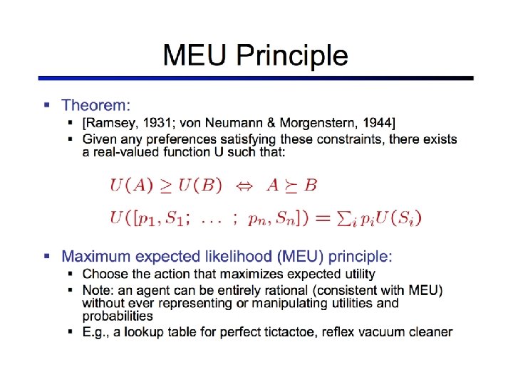
Why MEU?

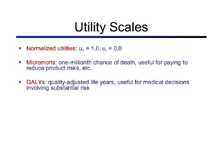
Human Utilities • How much do people value their lives? – How much would you pay to avoid a risk, e. g. Russian roulette with a million-barreled revolver (1 micromort)? – Driving in a car for 230 miles incurs a risk of 1 micromort.

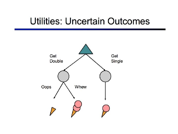
Measuring Utilities Best possible prize Worst possible catastrophe

Markov Decision Processes Stochastic, sequential environments (Chapter 17) Image credit: P. Abbeel and D. Klein

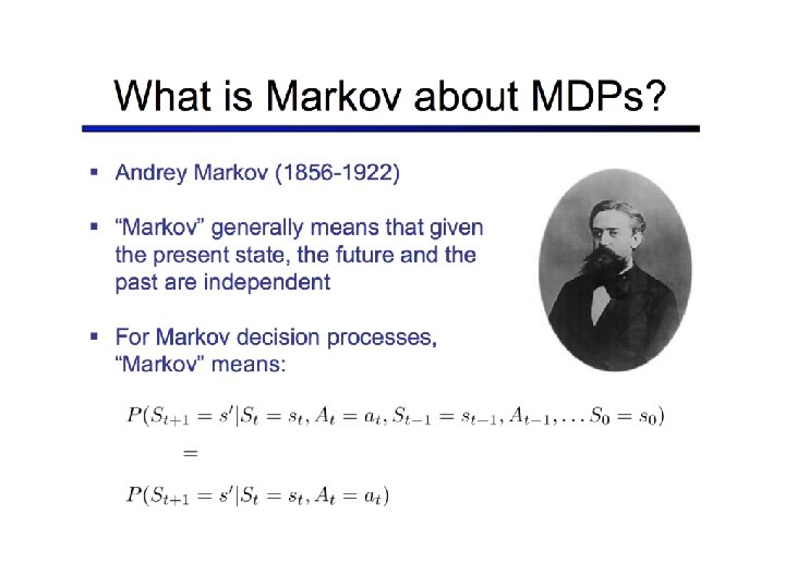
Markov Decision Processes • Components: – States s, beginning with initial state s 0 – Actions a • Each state s has actions A(s) available from it – Transition model P(s’ | s, a) • Markov assumption: the probability of going to s’ from s depends only on s and a and not on any other past actions or states – Reward function R(s) • Policy (s): the action that an agent takes in any given state – The “solution” to an MDP

Overview • First, we will look at how to “solve” MDPs, or find the optimal policy when the transition model and the reward function are known • Second, we will consider reinforcement learning, where we don’t know the rules of the environment or the consequences of our actions

Game show • A series of questions with increasing level of difficulty and increasing payoff • Decision: at each step, take your earnings and quit, or go for the next question – If you answer wrong, you lose everything $100 question Q 1 $1, 000 question Correct Q 2 $10, 000 question Correct Incorrect: $0 Quit: $100 $50, 000 question Correct Q 3 Q 4 Incorrect: $0 Quit: $1, 100 Correct: $61, 100 Incorrect: $0 Quit: $11, 100

Game show • Consider $50, 000 question – Probability of guessing correctly: 1/10 – Quit or go for the question? • What is the expected payoff for continuing? 0. 1 * 61, 100 + 0. 9 * 0 = 6, 110 • What is the optimal decision? $100 question Q 1 9/10 Correct $1, 000 question Q 2 3/4 Correct Incorrect: $0 Quit: $100 $10, 000 question 1/2 Correct Q 3 $50, 000 question Q 4 Incorrect: $0 Quit: $1, 100 1/10 Correct: $61, 100 Incorrect: $0 Quit: $11, 100

Game show • What should we do in Q 3? – Payoff for quitting: $1, 100 – Payoff for continuing: 0. 5 * $11, 100 = $5, 550 • What about Q 2? – $100 for quitting vs. $4, 162 for continuing • What about Q 1? U = $3, 746 U = $4, 162 $100 question $1, 000 question Q 1 9/10 Correct Q 2 3/4 Correct Incorrect: $0 Quit: $100 U = $5, 550 U = $11, 100 $10, 000 question $50, 000 question 1/2 Correct Q 3 Q 4 Incorrect: $0 Quit: $1, 100 1/10 Correct: $61, 100 Incorrect: $0 Quit: $11, 100

Grid world Transition model: 0. 1 0. 8 0. 1 R(s) = -0. 04 for every non-terminal state Source: P. Abbeel and D. Klein

Goal: Policy Source: P. Abbeel and D. Klein

Grid world Transition model: R(s) = -0. 04 for every non-terminal state

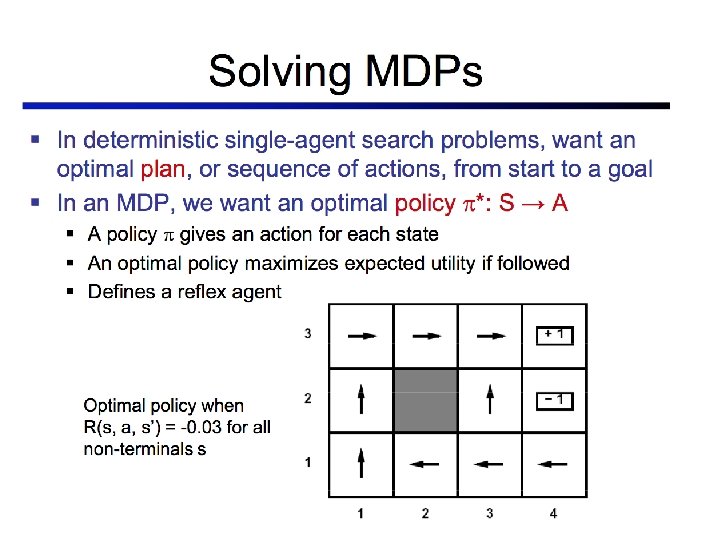
Grid world Optimal policy when R(s) = -0. 04 for every non-terminal state

Grid world • Optimal policies for other values of R(s):

Solving MDPs • MDP components: – States s – Actions a – Transition model P(s’ | s, a) – Reward function R(s) • The solution: – Policy (s): mapping from states to actions – How to find the optimal policy?

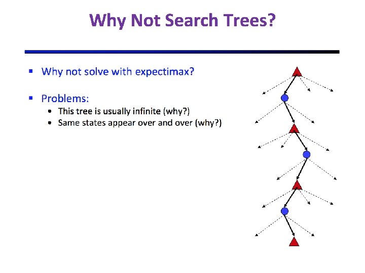
Maximizing expected utility • The optimal policy should maximize the expected utility over all possible state sequences produced by following that policy: • How to define the utility of a state sequence? – Sum of rewards of individual states – Problem: infinite state sequences

Utilities of state sequences • Normally, we would define the utility of a state sequence as the sum of the rewards of the individual states • Problem: infinite state sequences • Solution: discount the individual state rewards by a factor between 0 and 1: – Sooner rewards count more than later rewards – Makes sure the total utility stays bounded – Helps algorithms converge

Utilities of states • Expected utility obtained by policy starting in state s: • The “true” utility of a state, is the expected sum of discounted rewards if the agent executes an optimal policy starting in state s

Finding the utilities of states • What is the expected utility of taking action a in state s? Max node Chance node P(s’ | s, a) • How do we choose the optimal action? U(s’) • What is the recursive expression for U(s) in terms of the utilities of its successor states?

The Bellman equation • Recursive relationship between the utilities of successive states: Receive reward R(s) Choose optimal action a End up here with P(s’ | s, a) Get utility U(s’) (discounted by )

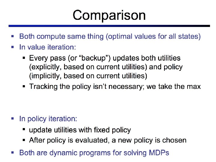
The Bellman equation • Recursive relationship between the utilities of successive states: • For N states, we get N equations in N unknowns – Solving them solves the MDP – We can solve them algebraically – Two methods: value iteration and policy iteration

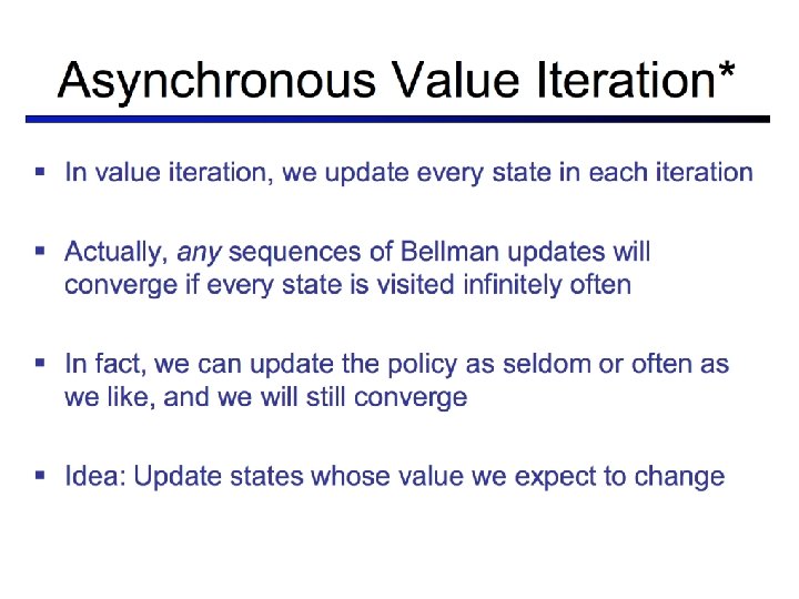
Method 1: Value iteration • Start out with every U(s) = 0 • Iterate until convergence – During the ith iteration, update the utility of each state according to this rule: • In the limit of infinitely many iterations, guaranteed to find the correct utility values – In practice, don’t need an infinite number of iterations…

Value iteration • What effect does the update have? Value iteration demo

Values vs Policy • Basic idea: approximations get refined towards optimal values • Policy may converge long before values do

Method 2: Policy iteration • Start with some initial policy 0 and alternate between the following steps: – Policy evaluation: calculate U i(s) for every state s – Policy improvement: calculate a new policy i+1 based on the updated utilities

Policy evaluation • Given a fixed policy , calculate U (s) for every state s • The Bellman equation for the optimal policy: – How does it need to change if our policy is fixed? – Can solve a linear system to get all the utilities! – Alternatively, can apply the following update:

Looking ahead

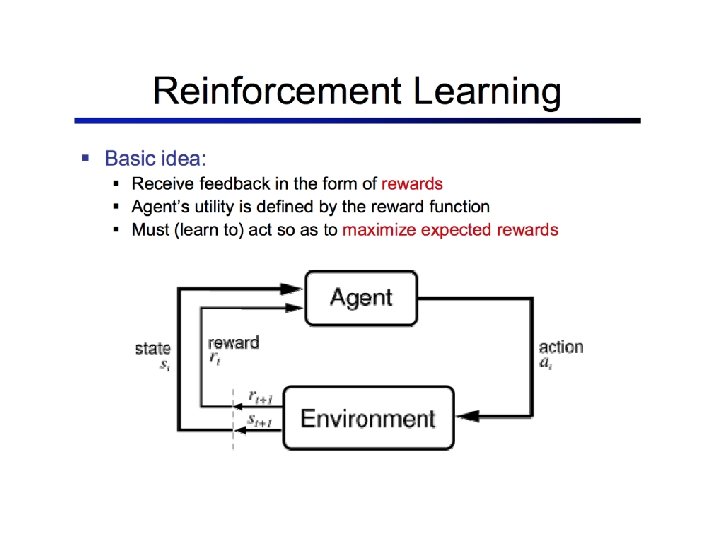
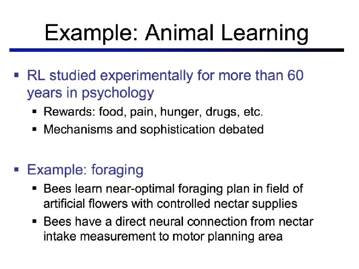
Reinforcement Learning • Components: – States s, beginning with initial state s 0 – Actions a • Each state s has actions A(s) available from it – Transition model P(s’ | s, a) – Reward function R(s) • Policy (s): the action that an agent takes in any given state – The “solution” • New twist: don’t know Transition model or Reward function ahead of time! – Have to actually try actions and states out to learn