Using Standardized Anomaly Data in Operational Forecasting Mike

Using Standardized Anomaly Data in Operational Forecasting Mike Bodner NCEP/HPC Development Training Branch Spring/Summer 2005

Training Outline • Overview of standard deviations and statistical methods in forecasting • Methodology and computational information behind operational standard deviations • Application of standard deviations for extreme temperature and heavy precipitation events • Suggested methodologies for local meso-scale standardized anomalies • Look at significant cases

We are already using tools that apply stochastic methods in operational forecasting… • MOS output • Ensembles • Short Range Ensemble Forecasts (SREFs)

Standard deviations can be another tool to add to the chest… • Based on 50 years of climatology • Can be applied to a model forecast output and assist in evaluating model trends

How are standard deviations generated? Daily averages and standard deviations (variances) are computed for the period 1950 -2003 from NCAR/NCEP Reanalysis data for • 500 h. Pa heights • 850 h. Pa temperatures • 1000 -500 h. Pa thickness and partial thicknesses

Another way of looking at it using 500 h. Pa heights… Standard deviation or σ is computed by the following formula. . σ = square root of the average of heights 2 - average height 2 The number of standard deviations from the climatology is computed by subtracting the 50 year average height from the model forecast or observed height then dividing by the standard deviation. Standardized Anomaly = (fcst height - average height) ÷ σ

• Reanalysis data is set on a 2. 5 x 2. 5 global grid domain • Model data is resized to coincide with the reanalysis domain

Keep in mind when looking at standard deviation data in an operational setting. . • Typically standardized anomalies of 3 -4 units from climatology during the cold season and 2 -3 in the warm season correspond with a significant temperature event • Forecast values of 5 and 6 are of extremely low probability and should be closely scrutinized if displayed in model forecast data

Rather benign day with not much going on

Surprise October 1996 snow event in Kansas City metro area. . 500 h. Pa heights were 4. 5 SDs lower than climatology

Other items to be aware of when using this tool • It’s beneficial to be aware of the standard deviations or at least the SD pattern for your forecast data • The climatological standard deviations are not as large over the southern latitudes, particularly during the warm season • Standard deviations are larger over the northern latitudes with the greatest variance over the North Pacific, North Atlantic and northeast North America.

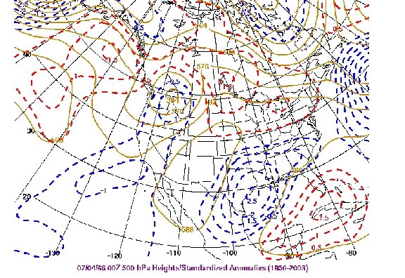
Here’s an example of the computed standard deviations for 500 h. Pa heights for July 4. Notice how the variance increases proportionally with latitude. Also note how the largest standard deviations occur over the North Pacific and North Atlantic.

Let’s apply the SD data from the July 4 image in the previous slide… • At Atlanta, GA. The average 500 h. Pa height for July 4 is 588 dm, and the standard deviation for 500 h. Pa height over Atlanta is 3 dm • A forecast value of 3 standard deviations from normal or -3 would suggest a forecast height of 579 dm which is 9 dm below climatology • At Seattle, WA. The average 500 h. Pa height for July 4 is about 570 dm, and the standard deviation for 500 h. Pa height over Seattle is 9 dm • A forecast value of 3 standard deviations from normal or -3 would suggest a forecast height of 543 dm or 27 dm below climatology.

As mentioned several slides earlier, height and temperature regimes depicted as 3 or more standard deviations from climatology are very rare. # of Standard Deviations Probability of Occurrence Based on Climatology 1σ 0. 6826895 2σ 0. 2718076 3σ 0. 0428032 4σ 0. 0026364 5σ 0. 0000628 The number of standard deviations are displayed with probability of occurrence of the number of standard deviations from climatology based on a standard probability density function (PDF) curve. The values include both above and below normal conditions.

The values plotted on the standard "bell curve" depict percent probability of a standard deviation being above or below the climatological mean (essentially these values are half of the probabilities sited in the above chart). As you can see, there is extremely low probability forecast events greater than 3 standard deviations from climatology. Also note that temperature events trend slightly to the left or colder than the median.

Let’s take a look a few regional heat cases… • Northeast U. S. Heat Wave – July 1966 • Central U. S. Heat Wave – July 1980 • Southwest U. S. Extreme Heat – June 1990

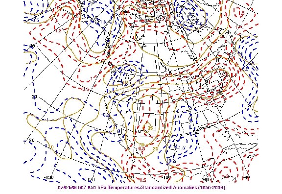
4 th of July Heat Wave over the Northeast U. S. Triple digit temperatures were noted over many Northeast locations during the 3 day period 3 -5 July 1966. On July 3, 1966, record high temperatures included 102 F at Hartford, CT, 107 F at La. Guardia (highest NYC area temperature), 105 F at Allentown, PA and 104 F at Philadelphia, PA. The 500 h. Pa charts for this record breaking heat event do not depict a pattern typical of a severe heat wave. 500 h. Pa heights are 2 standard deviations above climatology but the 850 h. Pa thermal field also ended up being a signal for this extreme temperature event.

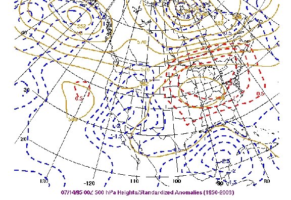
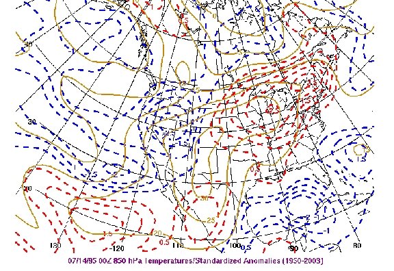
Chicago and Central U. S. Heat Wave 1995 On July 12 -15 a deadly heat wave effected the Chicago, IL and central U. S. Numerous triple digit temperatures were observed and several maximum temperature records were established during this event, particularly on July 13. Some record from this day included 106 F at Chicago Midway, 104 F at Chicago O’Hare, 103 F at Milwaukee, WI.

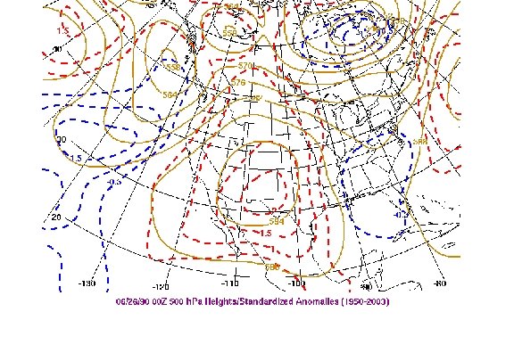
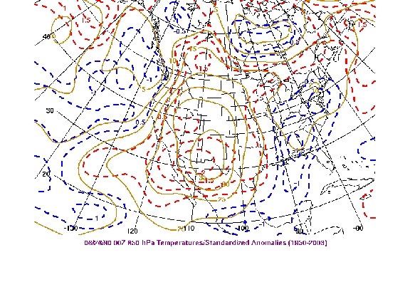
Southwest U. S. – Extreme Heat June 1990 A pre-monsoon 500 h. Pa anti-cyclone became established over the southwest U. S. in late June 1990. During the period June 25 -28, numerous records were set. On June 26, a record maximum temperature of 122 F was recorded at Phoenix, AZ. In Downtown Los Angeles a record 112 F was observed. Both 500 h. Pa heights and 850 h. Pa temperatures were 2 SDs above climatology near the center of the upper high.

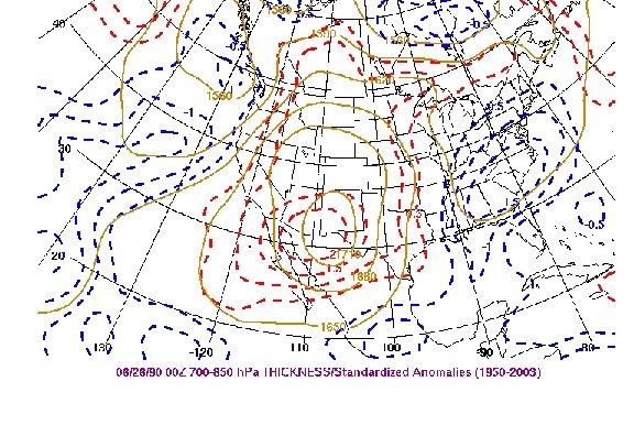
Note the close agreement of the 850 -700 h. Pa thickness with the 850 h. Pa temperature field. As with cold cases, this partial thickness may be used over high terrain where 850 h. Pa is negated.

Applying this tool to extreme cold at the regional scale… • Northeast U. S. – January 1994 • Central U. S. – November 1991 • Western U. S. – February 1989

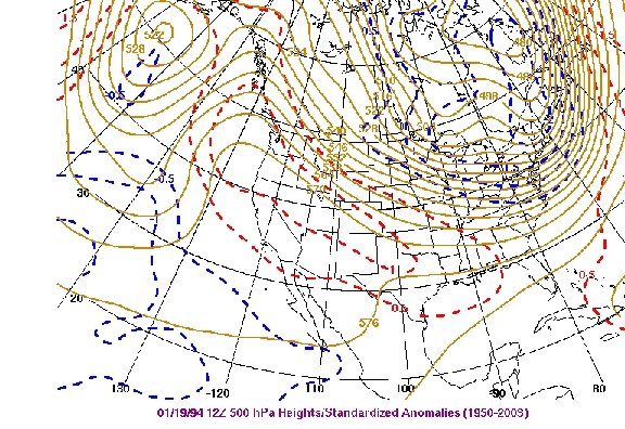
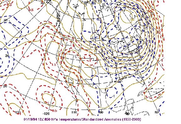
Record Cold Northeast U. S 19 -21 January 1994 Temperatures remained below zero for over 50 hours in Pittsburgh and many other sections of Pennsylvania, Ohio New York and New England during 19 -21 January 1994. 500 h. Pa height fields for 19 January 1994 show a deep trough over eastern North America, but the significant departure from climatology as depicted by the standard deviation fields illustrated the extent of the low level cold air. Moreover fresh snow cover increased the potential for an exceptionally cold boundary layer.

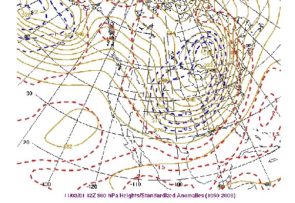
Record Cold over Central U. S. November 1991 Within days after the “perfect storm” churned up the western Atlantic and caused extensive damage to the Northeast coast, another intense cyclone resulted in an early season heavy snow event across the upper Mississippi Valley. In the aftermath of this storm, a full latitude trough delivered a record cold air mass to the plains states. Significant negative temperature anomalies were noted at 850 h. Pa. The images to the right show 500 and 850 h. Pa fields for 3 November 1991. This was the initial surge of arctic air into the central U. S. during a record breaking cold week.

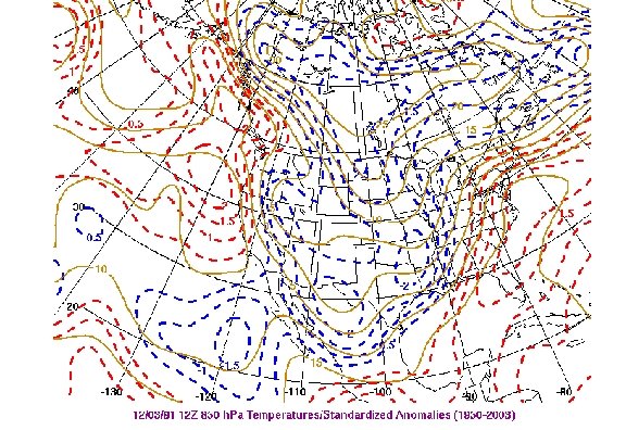
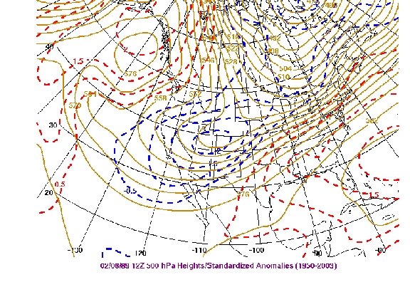
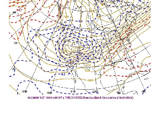
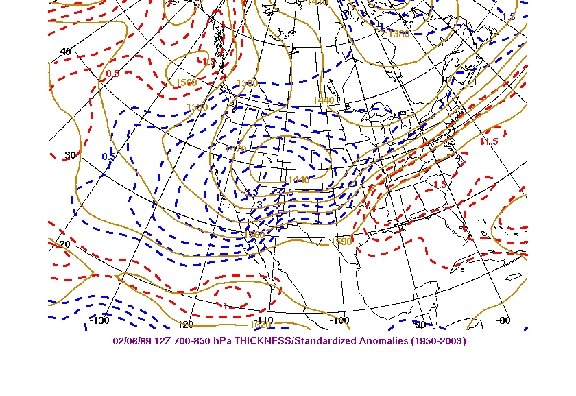
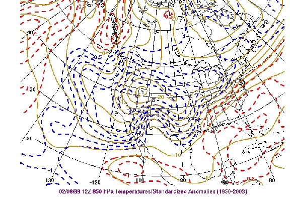
Record cold over Western U. S. February 1989 A very large arctic air mass moved into the western U. S. in early February 1989. The coldest anomalies both at 850 h. Pa and the surface were noted over the Great Basin region. Eventually the cold migrated to the central and southern plains. On the graphics for 6 February 1989, note the anomalously large ridge over the Gulf of Alaska at 500 h. Pa and full latitude trough over the western states to delivery the cold air. February records were set at Reno, NV, -15 F, -30 F at Ely, NV and 31 F at San Francisco, CA on 6 February 1989.

As was the case in the western heat event, since 850 h. Pa is “in the ground” over the intermountain region of the western U. S. , we can look at the 1000 -500 h. Pa and 850 -700 h. Pa thickness fields.

In spite of being “in the ground”, the 850 h. Pa temperature field correlates well with the record cold observed at the surface. Notice the -3. 0 to -3. 5 standardized anomalies over the lower elevations of California and the Central Plains.

Evaluating Model Data • Two summer cold front cases where fronts pushed unseasonably far to the south • 500 h. Pa heights examined to evaluate upper level thrust behind surface the cold fronts

Late July cold front into southern Texas

Look at model forecast

Early August cold front into Florida

Look at model forecasts

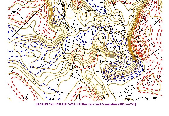
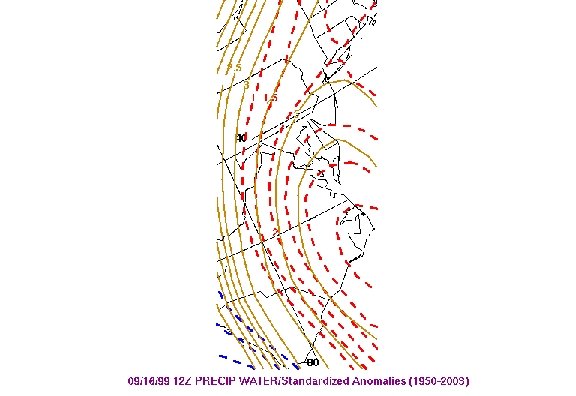
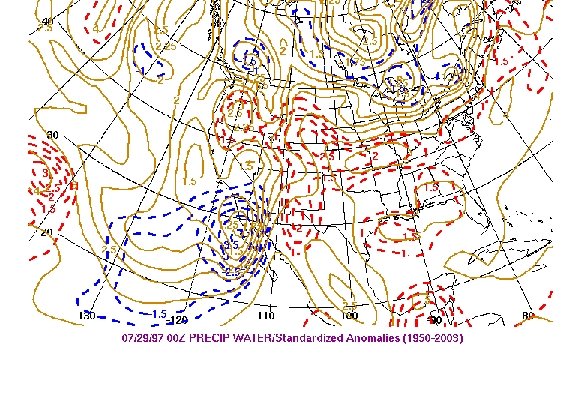
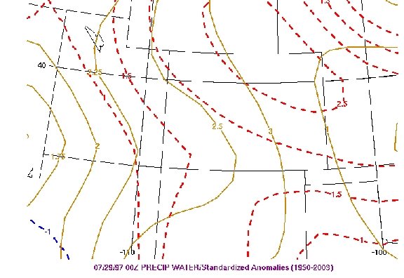
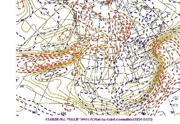
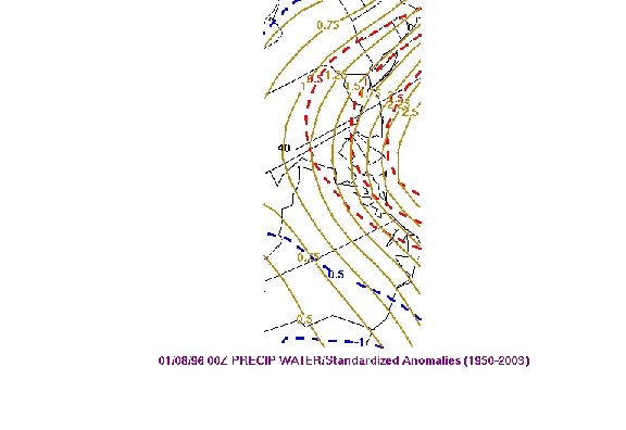
Heavy precipitation events… • Hurricane Floyd – September 1999 • Fort Collins, CO Flash Flood – July 1997 • Blizzard of 1996 – January 1996

When using standard deviations in the operational environment, always be mindful that… • It’s a statistical tool and not to be used to find an analogue from a “similar” past event. • Standardized anomalies are not a substitute for meteorological analysis, diagnosis and an informed forecast process. • Extreme standardized anomaly values may be an indicator that a particular model may be going astray or a significant trend is being detected by the model. • When applying standardized anomalies to temperature forecasting, local boundary layer conditions (i. e. snow cover and soil moisture) and cloud cover are not weighed into the calculation. • When applying standardized anomalies to heavy rainfall or winter weather scenarios, terrain effects and the influence of convective processes are not factored in.

More Operational Rules of Thumb • For a significant or record breaking event, a SD threshold of 2 is a guide for the warm season, and 3 for the cold season. • SDs >= 5 may be more an indication of model error than an extreme event. • Standardized anomalies of partial thicknesses do not show much skill in precipitation type forecasting but do show a signal for temperature events over the inter-mountain west.

Applying standardized anomalies to winter weather and heavy rainfall scenarios • A daily climatology may be too small a sample for events on the meso-scale • A pentad or greater time interval (as long as a month or half month) may be a better solution • A variance for specific humidity or mixing ratio can be computed for a specific event type, but often contain more statistical “noise” than the integrated precipitable water. i. e. a 50 year variance for specific humidity for northwest flow MCS events over the central U. S. during July 1 -15

Resources To view standard deviation data in real time, go to http: //www. hpc. ncep. noaa. gov/training/SDs/ To compute and display standard deviation for specific a specific date(s) over your CWA, the web site below is an excellent reference. http: //www. hpc. ncep. noaa. gov/ncepreanal Additional significant cases, including several on a more national scale can be found at the reference and training web site for using standard deviations. The web address is http: //www. hpc. noaa. gov/training If you have any questions or comments, please email mike. bodner@noaa. gov