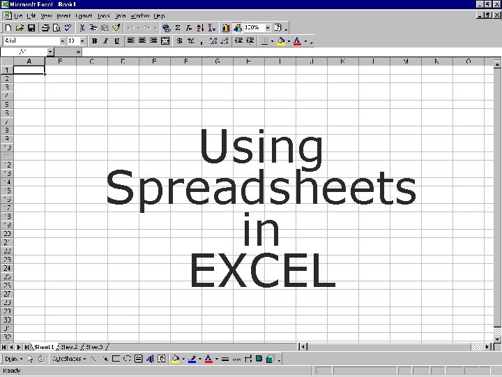
Using Spreadsheets in Excel Using Spreadsheets in EXCEL

Using Spreadsheets in Excel Using Spreadsheets in EXCEL

Uses of EXCEL Spreadsheets allow you to input, input manage and evaluate data. Within Excel you can: • enter data. • perform calculations using formulas. • create charts to illustrate data. • use functions to generate statistics.

The Excel Toolbars Save Print Format Painter Spell Check Print preview Open file Undo Auto Sum Redo Chart Wizard Draw Toolbar Function Insert Hyperlink Cut Zoom Sort Alphabetically Copy New file Paste Cell Border Cell Numbering Font Help Font Size Bold Underline Italic Merge Cells Alignment Percent Currency Indent Color Decimal Point Comma Background Text

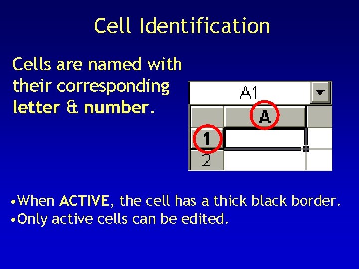
Cell Identification Cells are named with their corresponding letter & number • When ACTIVE, ACTIVE the cell has a thick black border. • Only active cells can be edited.

Naming a RANGE of Cells Groups of cells are referenced by: The top left corner & bottom right corner of the selection. B 2 D 7 You would write the expression like this: B 2: D 7

Referencing Cell Ranges How would you write the expression for this group of cells ? B 2: F 2

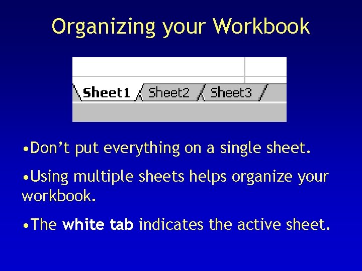
Organizing your Workbook • Don’t put everything on a single sheet. • Using multiple sheets helps organize your workbook. • The white tab indicates the active sheet.

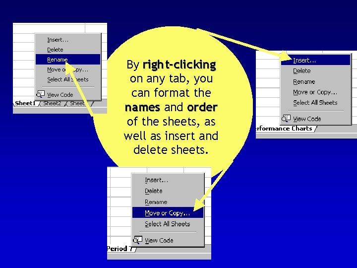
Renaming & Ordering Sheets By right-clicking on any tab, you can format the names and order of the sheets, as well as insert and delete sheets.

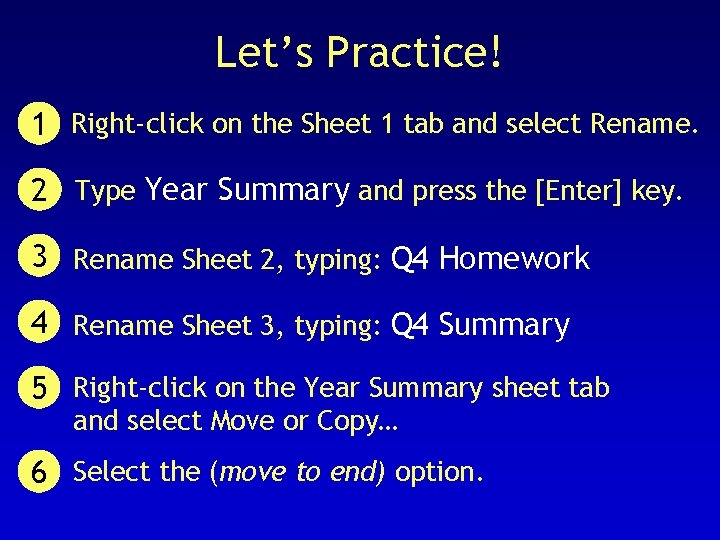
Let’s Practice! 1 Right-click on the Sheet 1 tab and select Rename. 2 Type Year Summary and press the [Enter] key. 3 Rename Sheet 2, typing: Q 4 Homework 4 Rename Sheet 3, typing: Q 4 Summary 5 Right-click on the Year Summary sheet tab and select Move or Copy… 6 Select the (move to end) option.

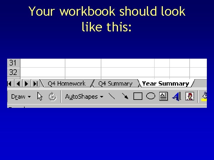
Your workbook should look like this:

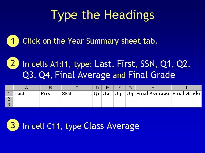
Type the Headings 1 Click on the Year Summary sheet tab. 2 In cells A 1: I 1, type: Last, First, SSN, Q 1, Q 2, Q 3, Q 4, Final Average and Final Grade 3 In cell C 11, type Class Average

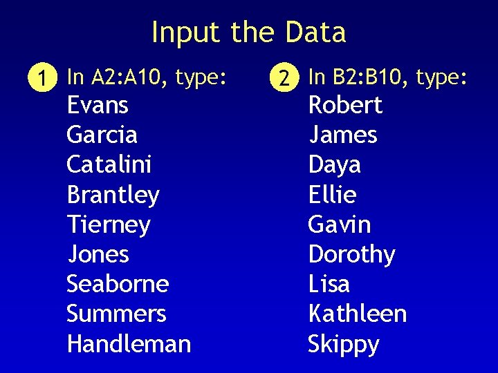
Input the Data 1 In A 2: A 10, type: Evans Garcia Catalini Brantley Tierney Jones Seaborne Summers Handleman 2 In B 2: B 10, type: Robert James Daya Ellie Gavin Dorothy Lisa Kathleen Skippy

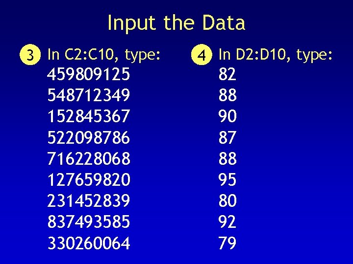
Input the Data 3 In C 2: C 10, type: 459809125 548712349 152845367 522098786 716228068 127659820 231452839 837493585 330260064 4 In D 2: D 10, type: 82 88 90 87 88 95 80 92 79

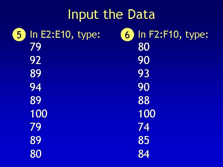
Input the Data 5 In E 2: E 10, type: 79 92 89 94 89 100 79 89 80 6 In F 2: F 10, type: 80 90 93 90 88 100 74 85 84

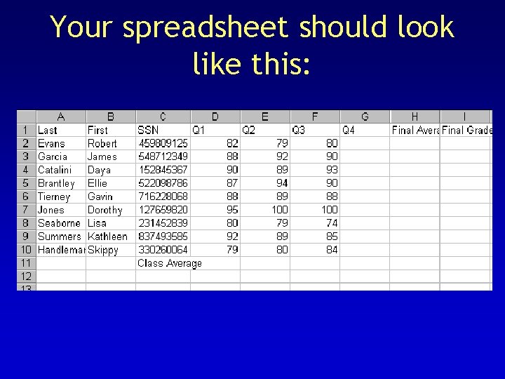
Your spreadsheet should look like this:

Using Formulas in Excel • A formula is used to calculate a value. • Formulas are created by combining: - Numbers. - Cell References. - Arithmetic Operators. - Functions.

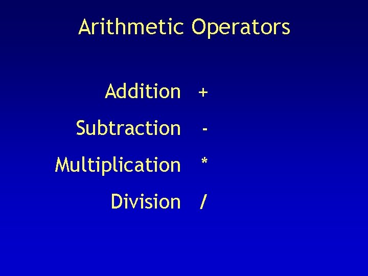
Arithmetic Operators Addition + Subtraction Multiplication * Division /

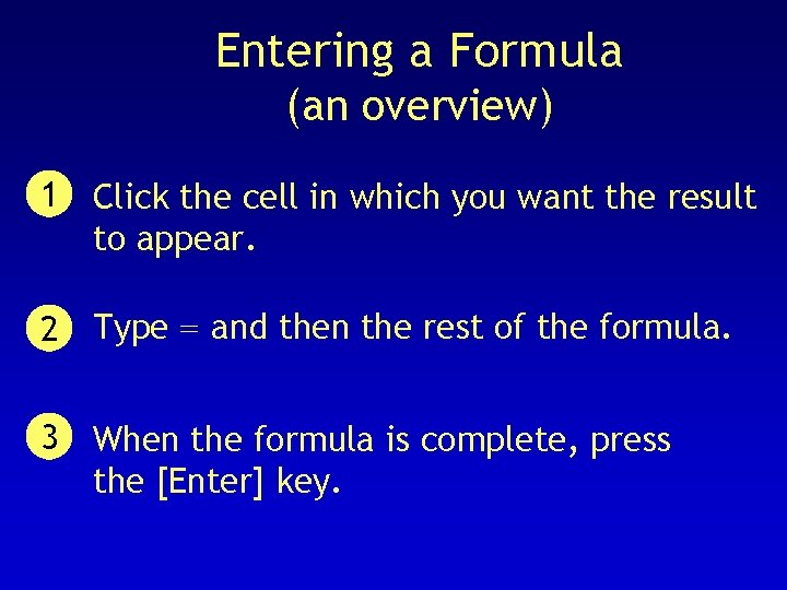
Entering a Formula (an overview) 1 Click the cell in which you want the result to appear. 2 Type = and then the rest of the formula. 3 When the formula is complete, press the [Enter] key.

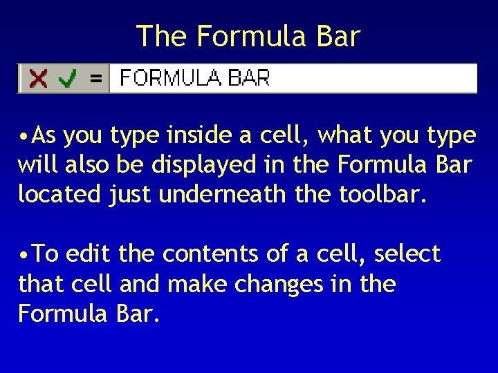
The Formula Bar • As you type inside a cell, what you type will also be displayed in the Formula Bar located just underneath the toolbar. • To edit the contents of a cell, select that cell and make changes in the Formula Bar.

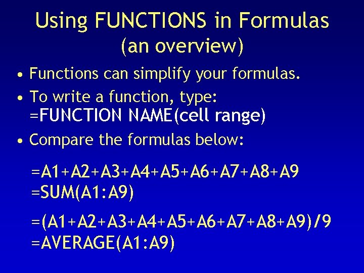
Using FUNCTIONS in Formulas (an overview) • Functions can simplify your formulas. • To write a function, type: =FUNCTION NAME(cell range) • Compare the formulas below: =A 1+A 2+A 3+A 4+A 5+A 6+A 7+A 8+A 9 =SUM(A 1: A 9) =(A 1+A 2+A 3+A 4+A 5+A 6+A 7+A 8+A 9)/9 =AVERAGE(A 1: A 9)

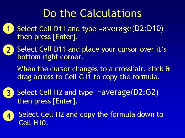
Copying the contents of cells To copy a formula or text: 1 Place the cursor over the bottom right corner of the cell, until the cursor turns into a crosshair. 2 Click and drag your mouse across or down to select the cells in which the formula will be pasted. Release the mouse.

Do the Calculations 1 Select Cell D 11 and type =average(D 2: D 10) then press [Enter]. 2 Select Cell D 11 and place your cursor over it’s bottom right corner. When the cursor changes to a crosshair, click & drag across to Cell G 11 to copy the formula. 3 Select Cell H 2 and type =average(D 2: G 2) then press [Enter]. 4 Select Cell H 2 and copy the formula down to Cell H 10.

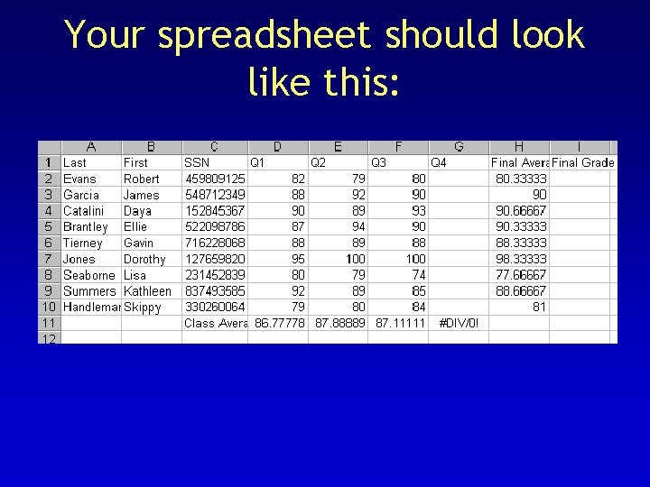
Your spreadsheet should look like this:

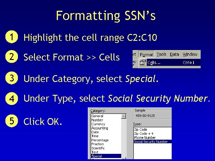
Formatting SSN’s 1 Highlight the cell range C 2: C 10 2 Select Format >> Cells 3 Under Category, select Special. 4 Under Type, select Social Security Number. 5 Click OK.

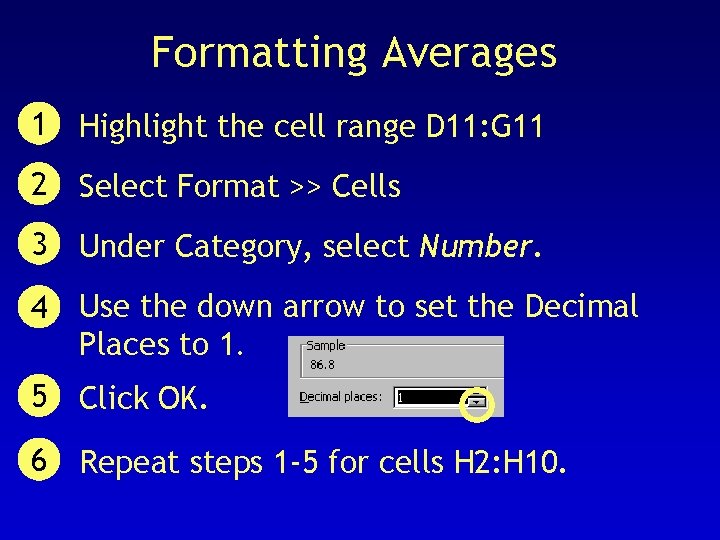
Formatting Averages 1 Highlight the cell range D 11: G 11 2 Select Format >> Cells 3 Under Category, select Number. 4 Use the down arrow to set the Decimal Places to 1. 5 Click OK. 6 Repeat steps 1 -5 for cells H 2: H 10.

The Little Extras 1 Select Cells A 1: I 1 and click the Bold icon on the Formatting toolbar. 2 Select Cell C 11 and bold that text as well. 3 Select A 1: I 1 again. Click the arrow next to the Border icon. Select the double border.

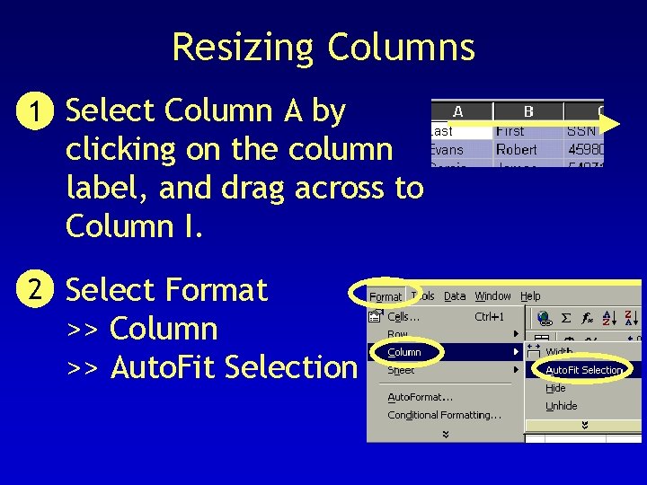
Resizing Columns 1 Select Column A by clicking on the column label, and drag across to Column I. 2 Select Format >> Column >> Auto. Fit Selection

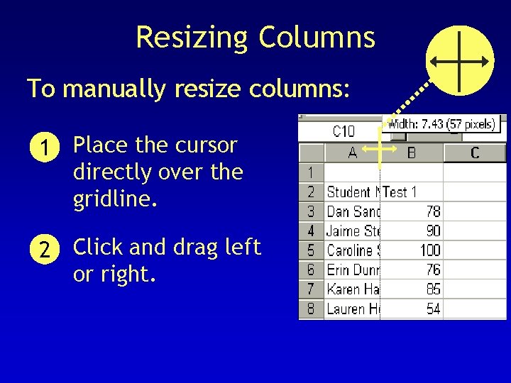
Resizing Columns To manually resize columns: 1 Place the cursor directly over the gridline. 2 Click and drag left or right.

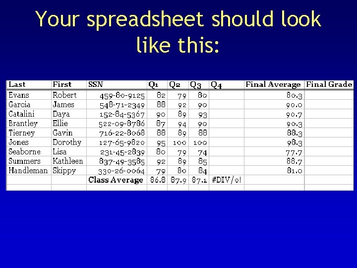
Your spreadsheet should look like this:

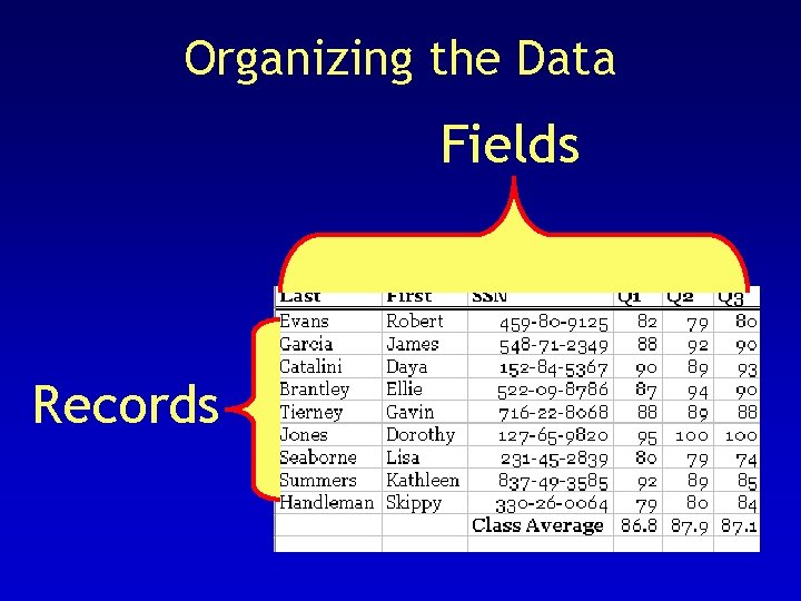
Organizing the Data Fields Records

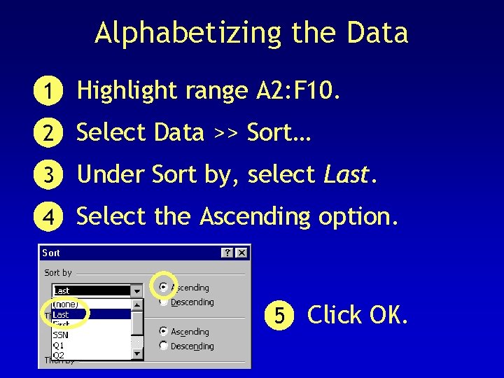
Alphabetizing the Data 1 Highlight range A 2: F 10. 2 Select Data >> Sort… 3 Under Sort by, select Last. 4 Select the Ascending option. 5 Click OK.

Working with Multiple Sheets 1 Highlight the cell range A 2: A 10. 2 Select Edit >> Copy. 3 Click on the Q 4 Homework sheet tab. 4 Click on Cell A 3. 5 Select Edit >> Paste. 6 Click on the Q 4 Summary sheet tab, and repeat Steps 4 & 5.

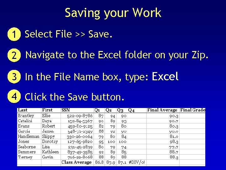
Saving your Work 1 Select File >> Save. 2 Navigate to the Excel folder on your Zip. 3 In the File Name box, type: Excel 4 Click the Save button.