Using SCHISM v Online manual and wiki resource

Using SCHISM v. Online manual and wiki resource: www. schism. wiki v. It helps if you know a few programming/scripting languages: python, matlab, FORTRAN/C… v. Bare minimum ØGenerate a hgrid. gr 3 with simplest possible b. c. ØRun SCHISM in 2 D config: manning. gr 3, param. in, bctides. in, vgrid. in ØPre-processing with ipre=1 first (with 1 CPU) to catch grid issues ØThen proceed to more complex set-ups 1

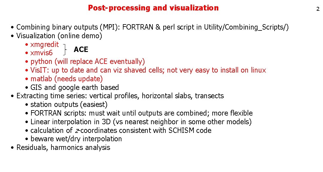
Post-processing and visualization • Combining binary outputs (MPI): FORTRAN & perl script in Utility/Combining_Scripts/) • Visualization (online demo) • xmgredit ACE • xmvis 6 • python (will replace ACE eventually) • Vis. IT: up to date and can viz shaved cells; not very easy to install on linux • matlab (needs update) • GIS and google earth based • Extracting time series: vertical profiles, horizontal slabs, transects • station outputs (easiest) • FORTRAN scripts: must wait until outputs are combined; more flexible • Linear interpolation in 3 D (vs nearest neighbor in some other models) • calculation of z-coordinates consistent with SCHISM code • beware wet/dry interpolation • Residuals, harmonics analysis 2

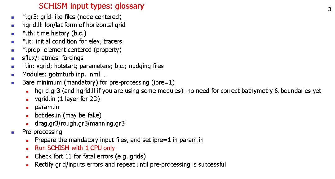
SCHISM input types: glossary n n n n n *. gr 3: grid-like files (node centered) hgrid. ll: lon/lat form of horizontal grid *. th: time history (b. c. ) *. ic: initial condition for elev, tracers *. prop: element centered (property) sflux/: atmos. forcings *. in: vgrid; hotstart; parameters; b. c. ; nudging files Modules: gotmturb. inp, . nml …. Bare minimum (mandatory) for pre-processing (ipre=1) n hgrid. gr 3 (and hgrid. ll if you are using some modules): no need for correct bathymetry & boundaries yet n vgrid. in (1 layer for 2 D) n param. in n bctides. in (may be fake) n drag. gr 3/rough. gr 3/manning. gr 3 Pre-processing n Prepare the mandatory input files, and set ipre=1 in param. in n Run SCHISM with 1 CPU only n Check fort. 11 for fatal errors (e. g. grids) n Rectify grid/inputs errors and repeat until pre-processing is successful 3

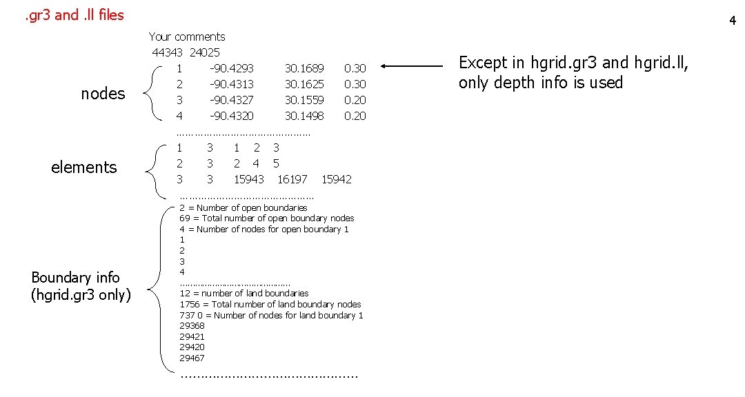
. gr 3 and. ll files nodes elements Boundary info (hgrid. gr 3 only) 4 Your comments 44343 24025 1 -90. 4293 30. 1689 0. 30 2 -90. 4313 30. 1625 0. 30 3 -90. 4327 30. 1559 0. 20 4 -90. 4320 30. 1498 0. 20 …………………… 1 3 1 2 3 2 4 5 3 3 15943 16197 15942 …………………… 2 = Number of open boundaries 69 = Total number of open boundary nodes 4 = Number of nodes for open boundary 1 1 2 3 4 …………………… 12 = number of land boundaries 1756 = Total number of land boundary nodes 737 0 = Number of nodes for land boundary 1 29368 29421 29420 29467 …………………… Except in hgrid. gr 3 and hgrid. ll, only depth info is used

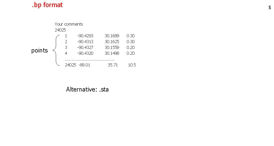
. bp format points 5 Your comments 24025 1 -90. 4293 30. 1689 0. 30 2 -90. 4313 30. 1625 0. 30 3 -90. 4327 30. 1559 0. 20 4 -90. 4320 30. 1498 0. 20 …………………… 24025 -89. 01 35. 71 10. 5 Alternative: . sta

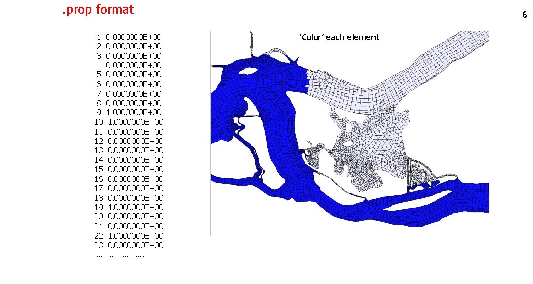
. prop format 1 0. 0000000 E+00 2 0. 0000000 E+00 3 0. 0000000 E+00 4 0. 0000000 E+00 5 0. 0000000 E+00 6 0. 0000000 E+00 7 0. 0000000 E+00 8 0. 0000000 E+00 9 1. 0000000 E+00 10 1. 0000000 E+00 11 0. 0000000 E+00 12 0. 0000000 E+00 13 0. 0000000 E+00 14 0. 0000000 E+00 15 0. 0000000 E+00 16 0. 0000000 E+00 17 0. 0000000 E+00 18 0. 0000000 E+00 19 1. 0000000 E+00 20 0. 0000000 E+00 21 0. 0000000 E+00 22 1. 0000000 E+00 23 0. 0000000 E+00 …………………. . 6 ‘Color’ each element

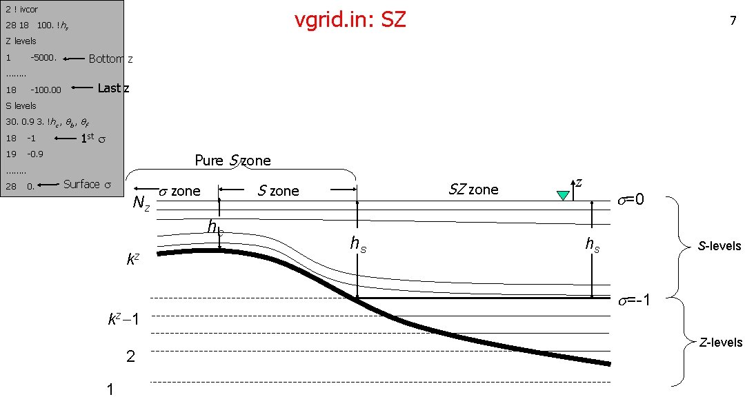
2 ! ivcor vgrid. in: SZ 28 18 100. !hs 7 Z levels 1 -5000. Bottom z -100. 00 Last z ……. . 18 S levels 30. 0. 9 3. !hc , qb , qf 18 -1 1 st s 19 -0. 9 Pure S zone ……. . 28 0. Surface s Nz s zone S zone hc kz kz-1 2 1 SZ zone hs z s=0 hs S-levels s=-1 Z-levels

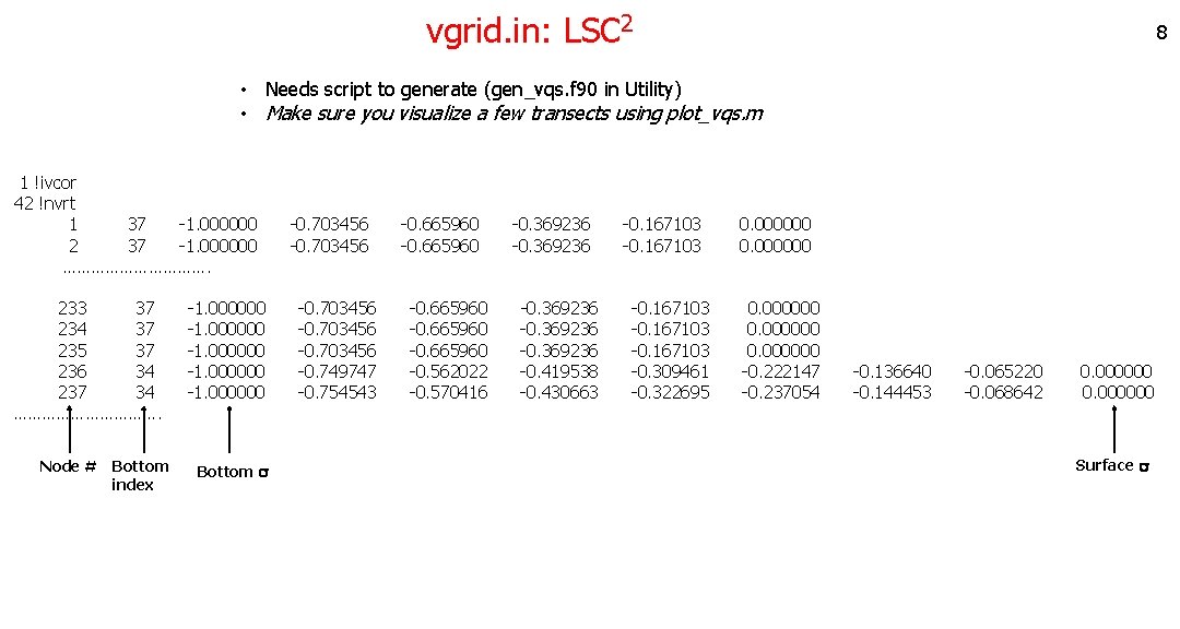
vgrid. in: LSC 2 8 • Needs script to generate (gen_vqs. f 90 in Utility) • Make sure you visualize a few transects using plot_vqs. m 1 !ivcor 42 !nvrt 1 37 -1. 000000 -0. 703456 -0. 665960 -0. 369236 -0. 167103 0. 000000 2 37 -1. 000000 -0. 703456 -0. 665960 -0. 369236 -0. 167103 0. 000000 ……………. 233 37 -1. 000000 -0. 703456 -0. 665960 -0. 369236 -0. 167103 0. 000000 234 37 -1. 000000 -0. 703456 -0. 665960 -0. 369236 -0. 167103 0. 000000 235 37 -1. 000000 -0. 703456 -0. 665960 -0. 369236 -0. 167103 0. 000000 236 34 -1. 000000 -0. 749747 -0. 562022 -0. 419538 -0. 309461 -0. 222147 -0. 136640 -0. 065220 0. 000000 237 34 -1. 000000 -0. 754543 -0. 570416 -0. 430663 -0. 322695 -0. 237054 -0. 144453 -0. 068642 0. 000000 ……………. Node # Bottom index Bottom s Surface s

bctides. in 04/15/2004 00: 00 PST 0 40. ntip 2 nbfr Z 0 0. 1. 0. O 1 6. 759775 e-05 1. 15343 118. 92151 4 nope 3 3 0 4 0 !Georgia Z 0 0. 1299680 0. 000000 E+00 O 1 0. 361010246 281. 862898 0. 36065857 281. 918305 0. 360767938 281. 968364 1. e-3 T relaxation 88 3 0 0 0 !ocean Z 0 8. 892417 E-02 0. 000000 E+00 8. 631096 E-02 0. 000000 E+00. . . O 1. . . 9 A simple example Extra b. c. flags for tracer models if invoked Phases don’t matter for Z 0 12/01/2013 00: 00 GMT 0 50. ntip 0 nbfr 2 !nope 1190 4 4 3 !Pacific 5. e-1 1. 139 4 4 3 !South China Sea 5. e-1 1. b. c. flag for enabled tracer module (SED in this case) • There is a way to cheat if you really cannot find the issue…. • B. C. flags drives additional inputs. th

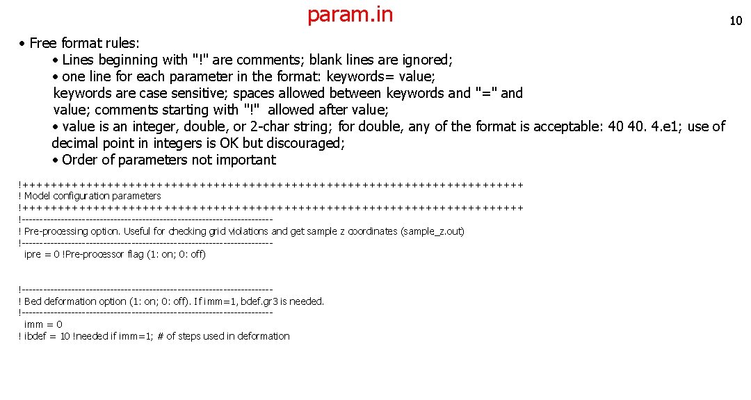
param. in 10 • Free format rules: • Lines beginning with "!" are comments; blank lines are ignored; • one line for each parameter in the format: keywords= value; keywords are case sensitive; spaces allowed between keywords and "=" and value; comments starting with "!" allowed after value; • value is an integer, double, or 2 -char string; for double, any of the format is acceptable: 40 40. 4. e 1; use of decimal point in integers is OK but discouraged; • Order of parameters not important !++++++++++++++++++++++++++++++++++++ ! Model configuration parameters !++++++++++++++++++++++++++++++++++++ !-----------------------------------! Pre-processing option. Useful for checking grid violations and get sample z coordinates (sample_z. out) !----------------------------------- ipre = 0 !Pre-processor flag (1: on; 0: off) !-----------------------------------! Bed deformation option (1: on; 0: off). If imm=1, bdef. gr 3 is needed. !----------------------------------- imm = 0 ! ibdef = 10 !needed if imm=1; # of steps used in deformation

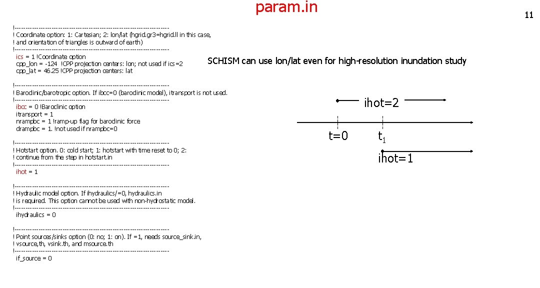
param. in 11 !-----------------------------------! Coordinate option: 1: Cartesian; 2: lon/lat (hgrid. gr 3=hgrid. ll in this case, ! and orientation of triangles is outward of earth) !----------------------------------- ics = 1 !Coordinate option SCHISM can use lon/lat even for high-resolution inundation study cpp_lon = -124 !CPP projection centers: lon; not used if ics=2 cpp_lat = 46. 25 !CPP projection centers: lat !-----------------------------------! Baroclinic/barotropic option. If ibcc=0 (baroclinic model), itransport is not used. !----------------------------------- ibcc = 0 !Baroclinic option itransport = 1 nrampbc = 1 !ramp-up flag for baroclinic force drampbc = 1. !not used if nrampbc=0 !-----------------------------------! Hotstart option. 0: cold start; 1: hotstart with time reset to 0; 2: ! continue from the step in hotstart. in !----------------------------------- ihot = 1 !-----------------------------------! Hydraulic model option. If ihydraulics/=0, hydraulics. in ! is required. This option cannot be used with non-hydrostatic model. !----------------------------------- ihydraulics = 0 !-----------------------------------! Point sources/sinks option (0: no; 1: on). If =1, needs source_sink. in, ! vsource, th, vsink. th, and msource. th !----------------------------------- if_source = 0 ihot=2 t=0 t 1 ihot=1

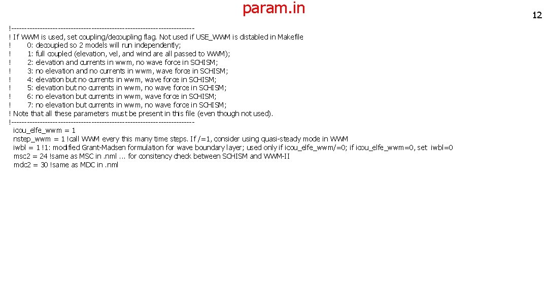
param. in !-----------------------------------! If WWM is used, set coupling/decoupling flag. Not used if USE_WWM is distabled in Makefile ! 0: decoupled so 2 models will run independently; ! 1: full coupled (elevation, vel, and wind are all passed to WWM); ! 2: elevation and currents in wwm, no wave force in SCHISM; ! 3: no elevation and no currents in wwm, wave force in SCHISM; ! 4: elevation but no currents in wwm, wave force in SCHISM; ! 5: elevation but no currents in wwm, no wave force in SCHISM; ! 6: no elevation but currents in wwm, wave force in SCHISM; ! 7: no elevation but currents in wwm, no wave force in SCHISM; ! Note that all these parameters must be present in this file (even though not used). !----------------------------------- icou_elfe_wwm = 1 nstep_wwm = 1 !call WWM every this many time steps. If /=1, consider using quasi-steady mode in WWM iwbl = 1 !1: modified Grant-Madsen formulation for wave boundary layer; used only if icou_elfe_wwm/=0; if icou_elfe_wwm=0, set iwbl=0 msc 2 = 24 !same as MSC in. nml. . . for consitency check between SCHISM and WWM-II mdc 2 = 30 !same as MDC in. nml 12

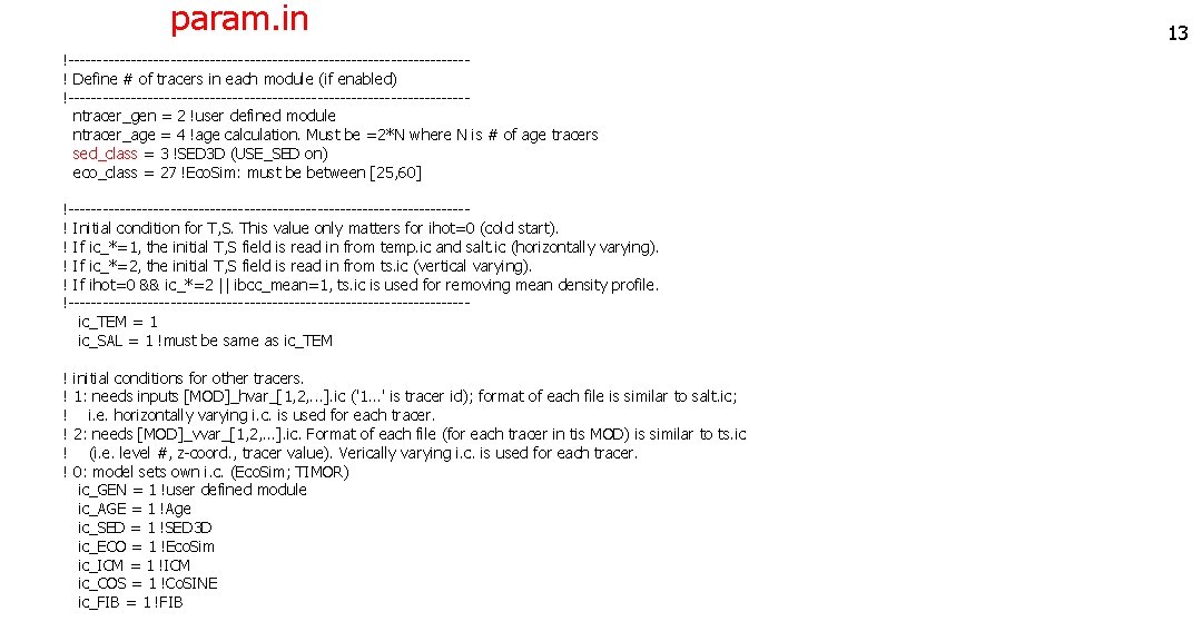
param. in !-----------------------------------! Define # of tracers in each module (if enabled) !----------------------------------- ntracer_gen = 2 !user defined module ntracer_age = 4 !age calculation. Must be =2*N where N is # of age tracers sed_class = 3 !SED 3 D (USE_SED on) eco_class = 27 !Eco. Sim: must be between [25, 60] !-----------------------------------! Initial condition for T, S. This value only matters for ihot=0 (cold start). ! If ic_*=1, the initial T, S field is read in from temp. ic and salt. ic (horizontally varying). ! If ic_*=2, the initial T, S field is read in from ts. ic (vertical varying). ! If ihot=0 && ic_*=2 || ibcc_mean=1, ts. ic is used for removing mean density profile. !----------------------------------- ic_TEM = 1 ic_SAL = 1 !must be same as ic_TEM ! initial conditions for other tracers. ! 1: needs inputs [MOD]_hvar_[1, 2, . . . ]. ic ('1. . . ' is tracer id); format of each file is similar to salt. ic; ! i. e. horizontally varying i. c. is used for each tracer. ! 2: needs [MOD]_vvar_[1, 2, . . . ]. ic. Format of each file (for each tracer in tis MOD) is similar to ts. ic ! (i. e. level #, z-coord. , tracer value). Verically varying i. c. is used for each tracer. ! 0: model sets own i. c. (Eco. Sim; TIMOR) ic_GEN = 1 !user defined module ic_AGE = 1 !Age ic_SED = 1 !SED 3 D ic_ECO = 1 !Eco. Sim ic_ICM = 1 !ICM ic_COS = 1 !Co. SINE ic_FIB = 1 !FIB 13

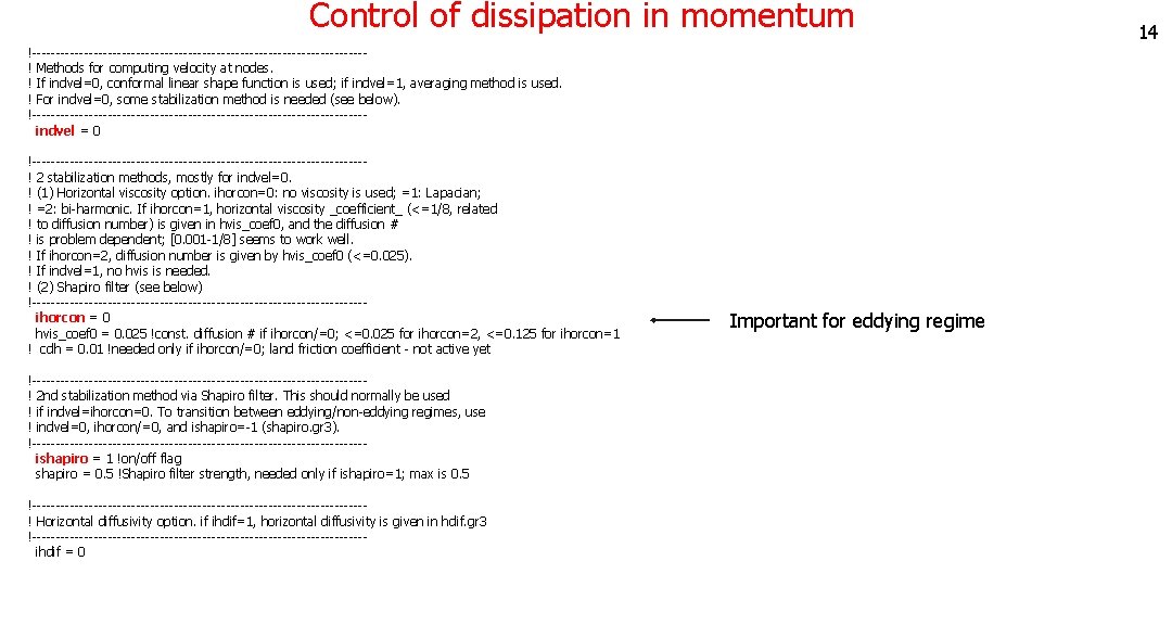
Control of dissipation in momentum !-----------------------------------! Methods for computing velocity at nodes. ! If indvel=0, conformal linear shape function is used; if indvel=1, averaging method is used. ! For indvel=0, some stabilization method is needed (see below). !----------------------------------- indvel = 0 !-----------------------------------! 2 stabilization methods, mostly for indvel=0. ! (1) Horizontal viscosity option. ihorcon=0: no viscosity is used; =1: Lapacian; ! =2: bi-harmonic. If ihorcon=1, horizontal viscosity _coefficient_ (<=1/8, related ! to diffusion number) is given in hvis_coef 0, and the diffusion # ! is problem dependent; [0. 001 -1/8] seems to work well. ! If ihorcon=2, diffusion number is given by hvis_coef 0 (<=0. 025). ! If indvel=1, no hvis is needed. ! (2) Shapiro filter (see below) !----------------------------------- ihorcon = 0 hvis_coef 0 = 0. 025 !const. diffusion # if ihorcon/=0; <=0. 025 for ihorcon=2, <=0. 125 for ihorcon=1 ! cdh = 0. 01 !needed only if ihorcon/=0; land friction coefficient - not active yet !-----------------------------------! 2 nd stabilization method via Shapiro filter. This should normally be used ! if indvel=ihorcon=0. To transition between eddying/non-eddying regimes, use ! indvel=0, ihorcon/=0, and ishapiro=-1 (shapiro. gr 3). !----------------------------------- ishapiro = 1 !on/off flag shapiro = 0. 5 !Shapiro filter strength, needed only if ishapiro=1; max is 0. 5 !-----------------------------------! Horizontal diffusivity option. if ihdif=1, horizontal diffusivity is given in hdif. gr 3 !----------------------------------- ihdif = 0 Important for eddying regime 14

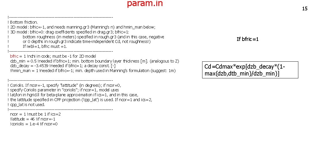
param. in !-----------------------------------! Bottom friction. ! 2 D model: bfric=-1, and needs manning. gr 3 (Manning's n) and hmin_man below; ! 3 D model: bfric=0: drag coefficients specified in drag. gr 3; bfric=1: ! bottom roughness (in meters) specified in rough. gr 3 (and in this case, negative ! or 0 depths in rough. gr 3 indicate time-independent Cd, not roughness!) ! If iwbl=1, bfric must =1. !----------------------------------- bfric = 1 !nchi in code; must be -1 for 2 D model dzb_min = 0. 5 !needed if bfric=1; min. bottom boundary layer thickness [m]. (analogous to Z) dzb_decay = -3. 4539 !needed if bfric=1; a decay const. [-] !hmin_man = 1 !needed if bfric=-1; min. depth used in Manning's formulation (suggest: 1 m) !-----------------------------------! Coriolis. If ncor=-1, specify "lattitude" (in degrees); if ncor=0, ! specify Coriolis parameter in "coriolis"; if ncor=1, model uses ! lat/lon in hgrid. ll for beta-plane approximation if ics=1, and in this case, ! the lattitude specified in CPP projection ('cpp_lat') is used. If ncor=1 and ics=2, ! cpp_lat is not used. !----------------------------------- ncor = 1 !must be 1 if ics=2 !latitude = 46 !if ncor=-1 !coriolis = 1. e-4 !if ncor=0 15 If bfric=1 Cd=Cdmax*exp[dzb_decay*(1 max(dzb, dtb_min)/dzb_min)]

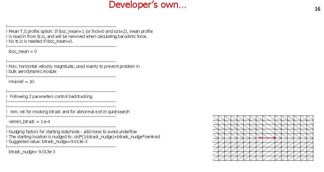
Developer’s own… !-----------------------------------! Mean T, S profile option. If ibcc_mean=1 (or ihot=0 and icst=2), mean profile ! is read in from ts. ic, and will be removed when calculating baroclinic force. ! No ts. ic is needed if ibcc_mean=0. !----------------------------------- ibcc_mean = 0 !-----------------------------------! Max. horizontal velocity magnitude, used mainly to prevent problem in ! bulk aerodynamic module !----------------------------------- rmaxvel = 10. !-----------------------------------! Following 2 parameters control backtracking !----------------------------------------------------------------------! min. vel for invoking btrack and for abnormal exit in quicksearch !----------------------------------- velmin_btrack = 1. e-4 !------------------------------------ ! Nudging factors for starting side/node - add noise to avoid underflow ! The starting location is nudged to: old*(1 -btrack_nudge)+btrack_nudge*centroid ! Suggested value: btrack_nudge=9. 013 e-3 !----------------------------------- btrack_nudge= 9. 013 e-3 16

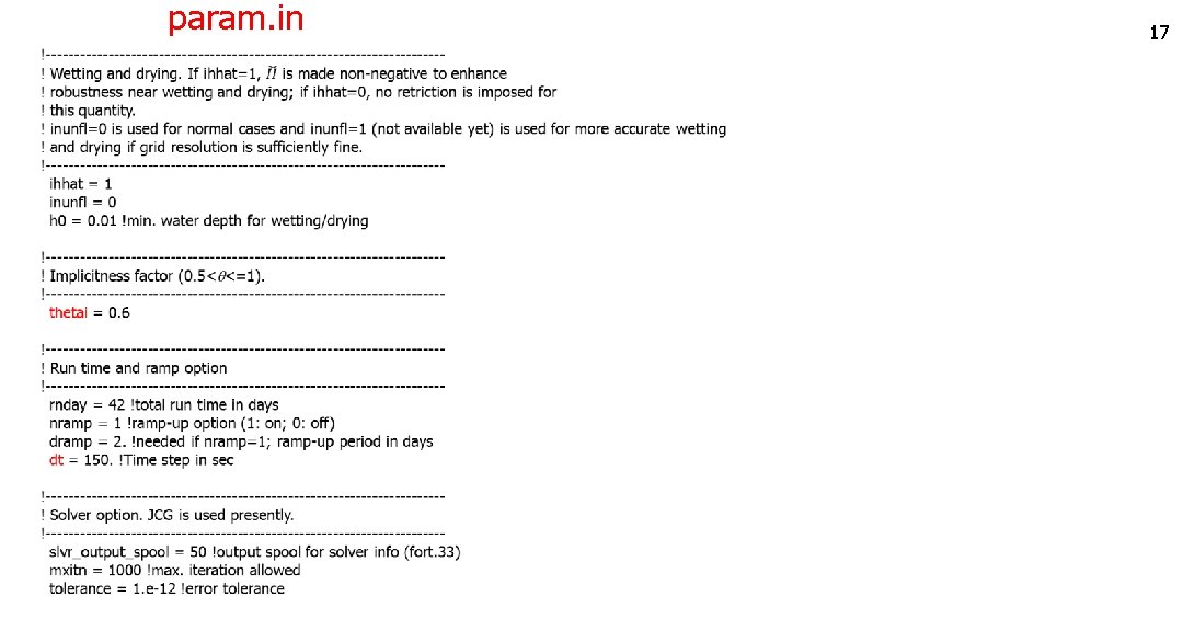
param. in 17

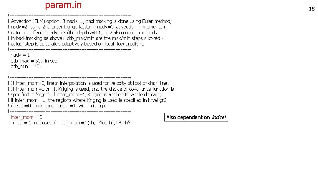
param. in !-----------------------------------! Advection (ELM) option. If nadv=1, backtracking is done using Euler method; ! nadv=2, using 2 nd order Runge-Kutta; if nadv=0, advection in momentum ! is turned off/on in adv. gr 3 (the depths=0, 1, or 2 also control methods ! in backtracking as above). dtb_max/min are the max/min steps allowed ! actual step is calculated adaptively based on local flow gradient. !----------------------------------- nadv = 1 dtb_max = 50. !in sec dtb_min = 15. !-----------------------------------! If inter_mom=0, linear interpolation is used for velocity at foot of char. line. ! If inter_mom=1 or -1, Kriging is used, and the choice of covariance function is ! specified in 'kr_co'. If inter_mom=1, Kriging is applied to whole domain; ! if inter_mom=-1, the regions where Kriging is used is specified in krvel. gr 3 ! (depth=0: no kriging; depth=1: with kriging). !----------------------------------- inter_mom = 0 Also dependent on indvel 2 3 5 kr_co = 1 !not used if inter_mom=0 (-h, h log(h), h , -h ) 18

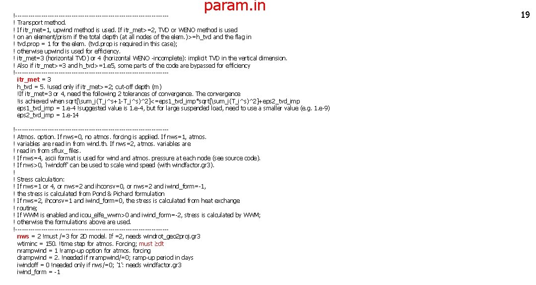
param. in !-----------------------------------! Transport method. ! If itr_met=1, upwind method is used. If itr_met>=2, TVD or WENO method is used ! on an element/prism if the total depth (at all nodes of the elem. )>=h_tvd and the flag in ! tvd. prop = 1 for the elem. (tvd. prop is required in this case); ! otherwise upwind is used for efficiency. ! itr_met=3 (horizontal TVD) or 4 (horizontal WENO -incomplete): implicit TVD in the vertical dimension. ! Also if itr_met>=3 and h_tvd>=1. e 5, some parts of the code are bypassed for efficiency !----------------------------------- itr_met = 3 h_tvd = 5. !used only if itr_met>=2; cut-off depth (m) !If itr_met=3 or 4, need the following 2 tolerances of convergence. The convergence !is achieved when sqrt[sum_i(T_i^s+1 -T_i^s)^2]<=eps 1_tvd_imp*sqrt[sum_i(T_i^s)^2]+eps 2_tvd_imp eps 1_tvd_imp = 1. e-4 !suggested value is 1. e-4, but for large suspended load, need to use a smaller value (e. g. 1. e-9) eps 2_tvd_imp = 1. e-14 !-----------------------------------! Atmos. option. If nws=0, no atmos. forcing is applied. If nws=1, atmos. ! variables are read in from wind. th. If nws=2, atmos. variables are ! read in from sflux_ files. ! If nws=4, ascii format is used for wind atmos. pressure at each node (see source code). ! If nws>0, 'iwindoff' can be used to scale wind speed (with windfactor. gr 3). ! ! Stress calculation: ! If nws=1 or 4, or nws=2 and ihconsv=0, or nws=2 and iwind_form=-1, ! the stress is calculated from Pond & Pichard formulation ! If nws=2, ihconsv=1 and iwind_form=0, the stress is calculated from heat exchange ! routine; ! If WWM is enabled and icou_elfe_wwm>0 and iwind_form=-2, stress is calculated by WWM; ! otherwise the formulations above are used. !----------------------------------- nws = 2 !must /=3 for 2 D model. If =2, needs windrot_geo 2 proj. gr 3 wtiminc = 150. !time step for atmos. Forcing; must ≥dt nrampwind = 1 !ramp-up option for atmos. forcing drampwind = 2. !needed if nrampwind/=0; ramp-up period in days iwindoff = 0 !needed only if nws/=0; '1': needs windfactor. gr 3 iwind_form = -1 19

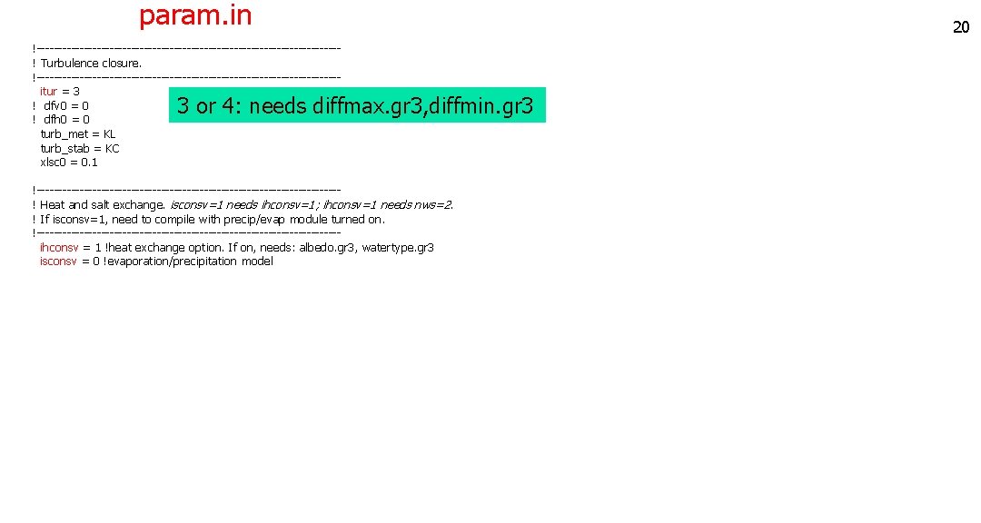
param. in !-----------------------------------! Turbulence closure. !----------------------------------- itur = 3 ! dfv 0 = 0 ! dfh 0 = 0 turb_met = KL turb_stab = KC xlsc 0 = 0. 1 3 or 4: needs diffmax. gr 3, diffmin. gr 3 !-----------------------------------! Heat and salt exchange. isconsv=1 needs ihconsv=1; ihconsv=1 needs nws=2. ! If isconsv=1, need to compile with precip/evap module turned on. !----------------------------------- ihconsv = 1 !heat exchange option. If on, needs: albedo. gr 3, watertype. gr 3 isconsv = 0 !evaporation/precipitation model 20

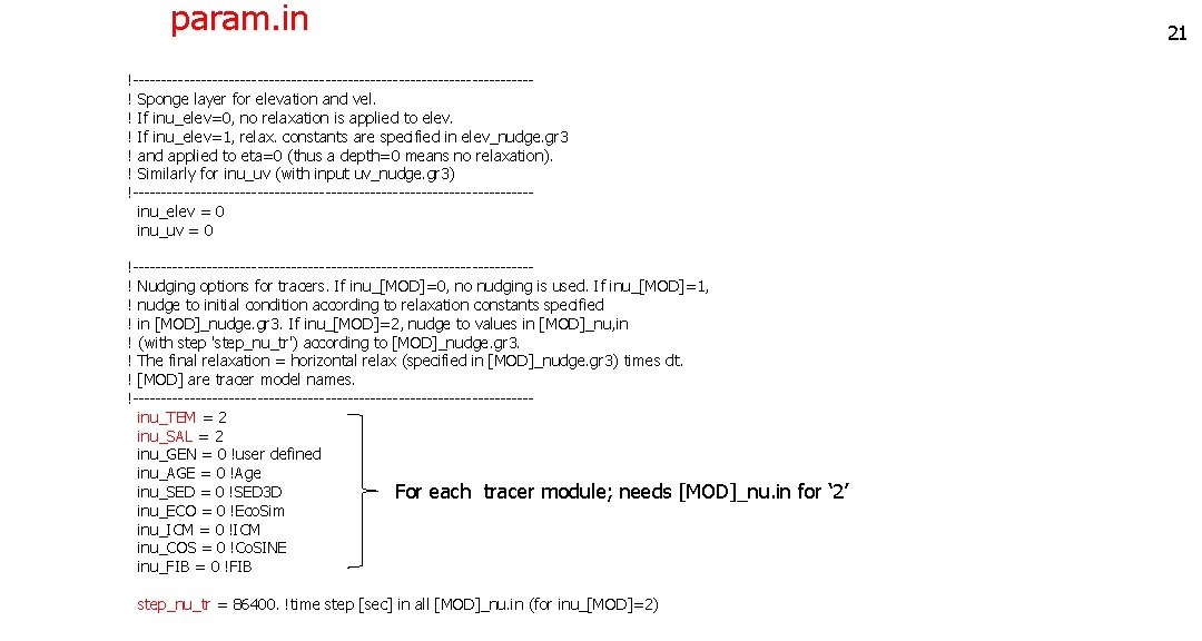
param. in !-----------------------------------! Sponge layer for elevation and vel. ! If inu_elev=0, no relaxation is applied to elev. ! If inu_elev=1, relax. constants are specified in elev_nudge. gr 3 ! and applied to eta=0 (thus a depth=0 means no relaxation). ! Similarly for inu_uv (with input uv_nudge. gr 3) !----------------------------------- inu_elev = 0 inu_uv = 0 !-----------------------------------! Nudging options for tracers. If inu_[MOD]=0, no nudging is used. If inu_[MOD]=1, ! nudge to initial condition according to relaxation constants specified ! in [MOD]_nudge. gr 3. If inu_[MOD]=2, nudge to values in [MOD]_nu, in ! (with step 'step_nu_tr') according to [MOD]_nudge. gr 3. ! The final relaxation = horizontal relax (specified in [MOD]_nudge. gr 3) times dt. ! [MOD] are tracer model names. !----------------------------------- inu_TEM = 2 inu_SAL = 2 inu_GEN = 0 !user defined inu_AGE = 0 !Age inu_SED = 0 !SED 3 D For each tracer module; needs [MOD]_nu. in for ‘ 2’ inu_ECO = 0 !Eco. Sim inu_ICM = 0 !ICM inu_COS = 0 !Co. SINE inu_FIB = 0 !FIB step_nu_tr = 86400. !time step [sec] in all [MOD]_nu. in (for inu_[MOD]=2) 21

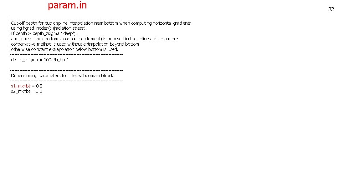
param. in !-----------------------------------! Cut-off depth for cubic spline interpolation near bottom when computing horizontal gradients ! using hgrad_nodes() (radiation stress). ! If depth > depth_zsigma ('deep'), ! a min. (e. g. max bottom z-cor for the element) is imposed in the spline and so a more ! conservative method is used without extrapolation beyond bottom; ! otherwise constant extrapolation below bottom is used. !----------------------------------- depth_zsigma = 100. !h_bcc 1 !-----------------------------------! Dimensioning parameters for inter-subdomain btrack. !----------------------------------- s 1_mxnbt = 0. 5 s 2_mxnbt = 3. 0 22

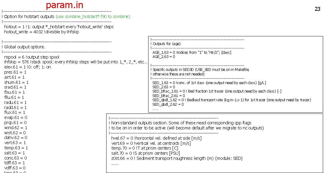
param. in 23 !-----------------------------------! Option for hotstart outputs (use combine_hotstart*. f 90 to combine) !----------------------------------- hotout = 1 !1: output *_hotstart every 'hotout_write' steps hotout_write = 4032 !divisible by ihfskip !------------------------------------ !-----------------------------------! Outputs for (age) ! Global output options. !---------------------------------------------------------------------- AGE_1. 63 = 0 !indices from "1" to "ntr/2"; [days] AGE_2. 63 = 0 nspool = 6 !output step spool ihfskip = 576 !stack spool; every ihfskip steps will be put into 1_*, 2_*, etc. . . !----------------------------------- elev. 61 = 1 !0: off; 1: on ! Specific outputs in SED 3 D (USE_SED must be on in Makefile; pres. 61 = 1 ! otherwise these are not needed) airt. 61 = 1 !----------------------------------- shum. 61 = 1 SED_1. 63 = 0 !conc. of 1 st class (one output need by each class) [g/L] SED_2. 63 = 0 srad. 61 = 1 SED_bfrac_1. 61 = 0 ! Bed fraction 1 st tracer (one output need by each class) [-] flsu. 61 = 1 SED_bfrac_2. 61 = 0 fllu. 61 = 1 SED_qbdl_1. 62 = 0 ! Bedload transport rate (kg. m-1. s-1) for 1 st tracer (one output need by tracer) radu. 61 = 1 SED_qbdl_2. 62 = 0 radd. 61 = 1 …… flux. 61 = 1 evap. 61 = 0 !----------------------------------- prcp. 61 = 0 ! Non-standard outputs section. Some of these need corresponding cpp flags wind. 62 = 1 ! to be on in order to be active (will become default after we migrate to nc outputs) wist. 62 = 0 !----------------------------------- dahv. 62 = 0 hvel. 67 = 0 !horizontal vel. defined at side [m/s] vert. 63 = 1 vert. 69 = 0 !vertical vel. at centroids [m/s] temp. 63 = 1 temp. 70 = 0 !T at prism centers [C] salt. 63 = 1 salt. 70 = 0 !S at prism centers [PSU] conc. 63 = 0 z 0 st. 66 = 0 ! Sediment transport roughness length (m) {module: SED} tdff. 63 = 1 …… vdff. 63 = 0

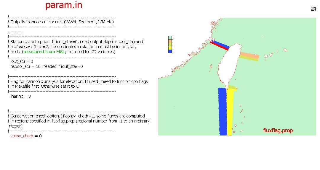
param. in 24 !-----------------------------------! Outputs from other modules (WWM, Sediment, ICM etc) !-----------------------------------…………. !-----------------------------------! Station output option. If iout_sta/=0, need output skip (nspool_sta) and ! a station. in. If ics=2, the cordinates in station. in must be in lon. , lat, ! and z (measured from MSL; not used for 2 D variables). !----------------------------------- iout_sta = 0 nspool_sta = 10 !needed if iout_sta/=0 !-----------------------------------! Flag for harmonic analysis for elevation. If used , need to turn on cpp flags ! in Makefile first. Otherwise set it to 0. !----------------------------------- iharind = 0 !-----------------------------------! Conservation check option. If consv_check=1, some fluxes are computed ! in regions specified in fluxflag. prop (regional number from -1 to an arbitrary integer). !----------------------------------- consv_check = 0 fluxflag. prop

Most important parameters are… • Momentum dissipation: indvel, ihorcon, ishapiro, inter_mom • Appropriate combination of these must be used for different applications (dispersion vs diffusion) • May start with: indvel= ihorcon=inter_mom=0, ishapiro=1 (‘MB-LI’ scheme) • If diffusion is still too high, use indvel= inter_mom=ishapiro=0, ihorcon=2, hvis_coef 0=0. 025 (or smaller) – the ‘eddying’ option. If oscillation is found in non-eddying part, use ishapiro=-1 and set the filter strength in shapiro. gr 3 • indvel=1 (ihorcon=ishapiro=inter_mom=0) is the most diffusive option (‘MA-LI’ scheme), but can be useful for 2 D runs e. g. • dt: appropriate time step (another way to control dispersion/diffusion) • nws: use ‘ 2’ as much as possible (and there are scripts for generating sflux*. nc) • itr_met: use 3 and ‘h_tvd’ and tvd. prop to control efficiency

Hotstart. in (unformatted binary) read(36) double 1, iths, ifile ! Element data do i=1, ne_global read(36) iegb, idry_e, (we(j, i), trel(1: ntracers, j, i), j=1, nvrt) enddo !i=1, ne_global ! Side data (side info can be generated by schism_geometry. f 90) do i=1, ns_global read(36) isgb, idry_s, (su 2(j, i), sv 2(j, i), tsd(j, i), ssd(j, i), j=1, nvrt) enddo ! Node data do i=1, np_global read(36) ipgb, eta 2, idry, (tr_nd(1: ntracers, j, i), tr_nd 0 (1: ntracers, j, i), q 2(i, j), xl(i, j), dfv(i, j), dfh(i, j), dfq 1(i, j), dfq 2(i, j), qnon(i, j), j=1, nvrt) enddo !Optional modules data (ICM, SED 2 D, HA) Nudging (TEM_nu. in and SAL_nu. in) (unformatted binary) do it=1, n_nudging_steps read(35) time_stamp !from t=0 do i=1, np_global read(35)temp_nu(1: nvrt, i) enddo !it 26

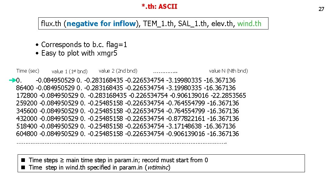
*. th: ASCII 27 flux. th (negative for inflow), TEM_1. th, SAL_1. th, elev. th, wind. th • Corresponds to b. c. flag=1 • Easy to plot with xmgr 5 Time (sec) value 1 (1 st bnd) value 2 (2 nd bnd) …………. . value N (Nth bnd) 0. -0. 084950529 0. -0. 283168435 -0. 226534754 -3. 19980335 -16. 367136 86400 -0. 084950529 0. -0. 283168435 -0. 226534754 -3. 19980335 -16. 367136 172800 -0. 084950529 0. -0. 283168435 -0. 226534754 -0. 906139016 -22. 2853565 259200 -0. 084950529 0. -0. 25485158 -0. 226534754 -0. 764554799 -16. 367136 345600 -0. 084950529 0. -0. 25485158 -0. 226534754 -0. 764554799 -16. 367136 432000 -0. 084950529 0. -0. 25485158 -0. 226534754 -0. 877822161 -16. 367136 518400 -0. 084950529 0. -0. 25485158 -0. 226534754 -3. 17148638 -16. 367136 604800 -0. 084950529 0. -0. 25485158 -0. 226534754 -0. 906139016 -16. 367136 ……………………………………………………. n Time steps ≥ main time step in param. in; record must start from 0 n Time step in wind. th specified in param. in (wtiminc)

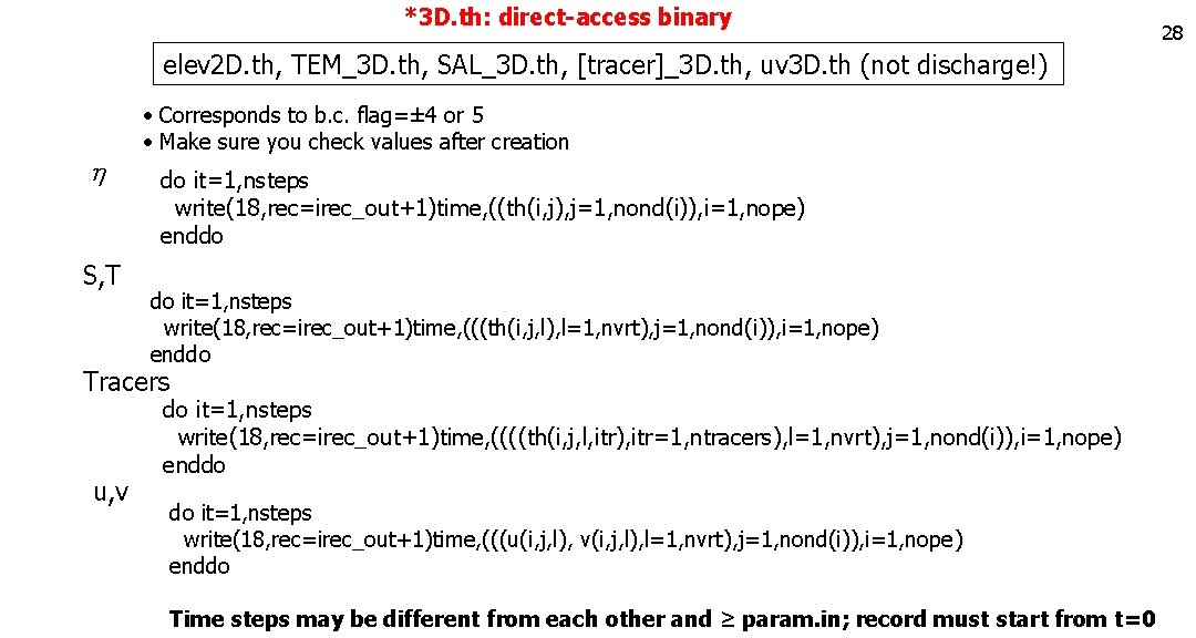
*3 D. th: direct-access binary elev 2 D. th, TEM_3 D. th, SAL_3 D. th, [tracer]_3 D. th, uv 3 D. th (not discharge!) h S, T • Corresponds to b. c. flag=± 4 or 5 • Make sure you check values after creation do it=1, nsteps write(18, rec=irec_out+1)time, ((th(i, j), j=1, nond(i)), i=1, nope) enddo do it=1, nsteps write(18, rec=irec_out+1)time, (((th(i, j, l), l=1, nvrt), j=1, nond(i)), i=1, nope) enddo Tracers u, v do it=1, nsteps write(18, rec=irec_out+1)time, ((((th(i, j, l, itr), itr=1, ntracers), l=1, nvrt), j=1, nond(i)), i=1, nope) enddo do it=1, nsteps write(18, rec=irec_out+1)time, (((u(i, j, l), v(i, j, l), l=1, nvrt), j=1, nond(i)), i=1, nope) enddo Time steps may be different from each other and ≥ param. in; record must start from t=0 28

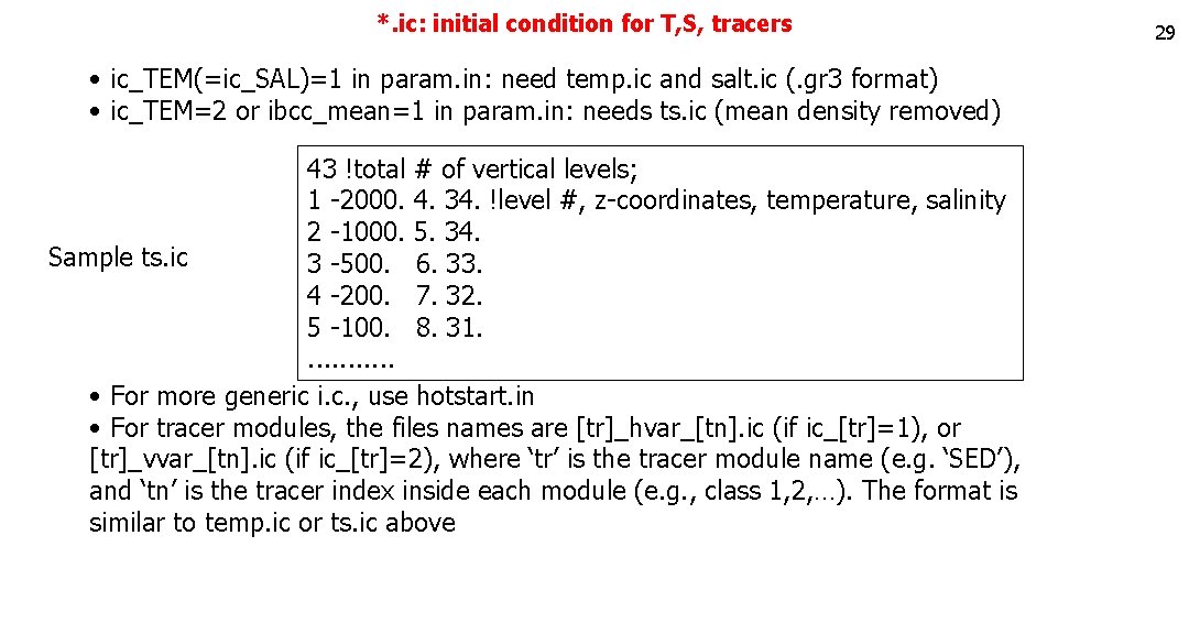
*. ic: initial condition for T, S, tracers • ic_TEM(=ic_SAL)=1 in param. in: need temp. ic and salt. ic (. gr 3 format) • ic_TEM=2 or ibcc_mean=1 in param. in: needs ts. ic (mean density removed) 43 !total # of vertical levels; 1 -2000. 4. 34. !level #, z-coordinates, temperature, salinity 2 -1000. 5. 34. Sample ts. ic 3 -500. 6. 33. 4 -200. 7. 32. 5 -100. 8. 31. . . • For more generic i. c. , use hotstart. in • For tracer modules, the files names are [tr]_hvar_[tn]. ic (if ic_[tr]=1), or [tr]_vvar_[tn]. ic (if ic_[tr]=2), where ‘tr’ is the tracer module name (e. g. ‘SED’), and ‘tn’ is the tracer index inside each module (e. g. , class 1, 2, …). The format is similar to temp. ic or ts. ic above 29

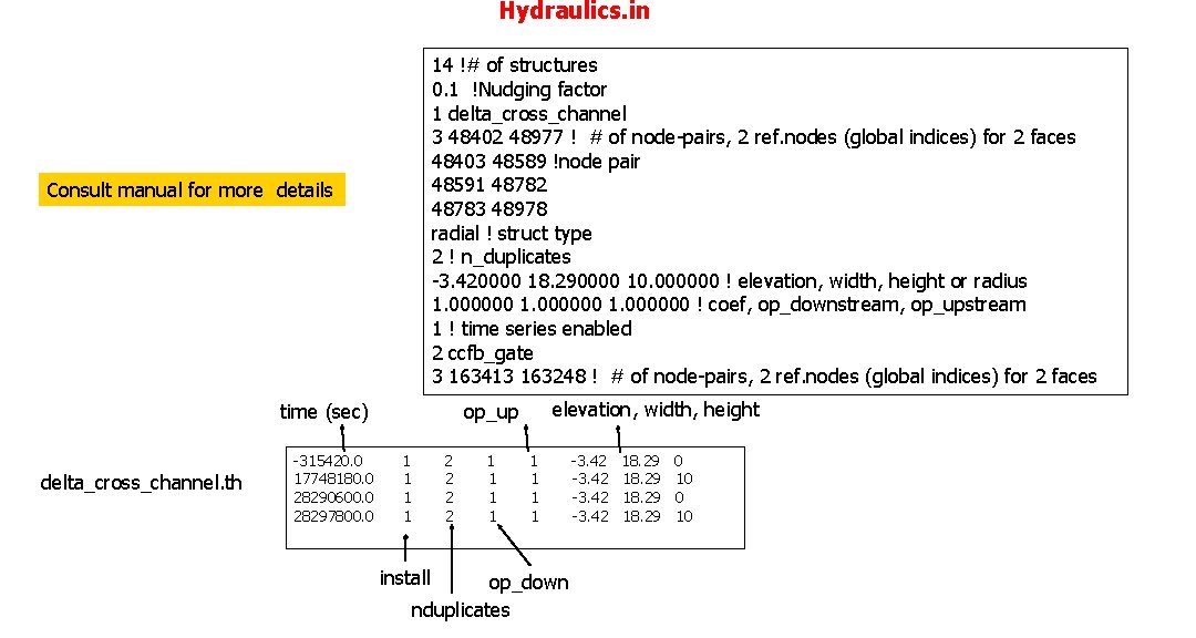
Hydraulics. in 14 !# of structures 0. 1 !Nudging factor 1 delta_cross_channel 3 48402 48977 ! # of node-pairs, 2 ref. nodes (global indices) for 2 faces 48403 48589 !node pair 48591 48782 48783 48978 radial ! struct type 2 ! n_duplicates -3. 420000 18. 290000 10. 000000 ! elevation, width, height or radius 1. 000000 ! coef, op_downstream, op_upstream 1 ! time series enabled 2 ccfb_gate 3 163413 163248 ! # of node-pairs, 2 ref. nodes (global indices) for 2 faces Consult manual for more details time (sec) delta_cross_channel. th op_up elevation, width, height -315420. 0 1 2 1 1 -3. 42 18. 29 0 17748180. 0 1 2 1 1 -3. 42 18. 29 10 28290600. 0 1 2 1 1 -3. 42 18. 29 0 28297800. 0 1 2 1 1 -3. 42 18. 29 10 install op_down nduplicates

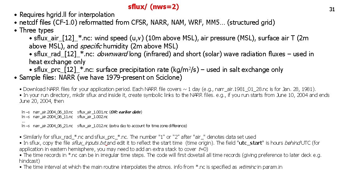
sflux/ (nws=2) • Requires hgrid. ll for interpolation • netcdf files (CF-1. 0) reformatted from CFSR, NARR, NAM, WRF, MM 5… (structured grid) • Three types • sflux_air_[12]_*. nc: wind speed (u, v) (10 m above MSL), air pressure (MSL), surface air T (2 m above MSL), and specific humidity (2 m above MSL) • sflux_rad_[12]_*. nc: downward long (infrared) and short (solar) wave radiation fluxes – used in heat exchange only • sflux_prc_[12]_*. nc: surface precipitation rate (kg/m 2/s) – used in salt exchange only • Sample files: NARR (we have 1979 -present on Sciclone) 31 • Download NARR files for your application period. Each NARR file covers ~ 1 day (e. g. , narr_air. 1981_01_28. nc is for Jan. 28, 1981). • In your run directory, mkdir sflux and inside it, create symbolic links to the NARR files. e. g. , if you run starts from June 10, 2004 and ends June 20, 2004, then ln –s narr_air. 2004_06_10. nc sflux_air_1. 001. nc (OR: earlier date) ln –s narr_air. 2004_06_11. nc sflux_air_1. 002. nc . . . ln –s narr_air. 2004_06_21. nc sflux_air_1. 012. nc (extra day to account for time zone difference) • Similarly for sflux_rad_*. nc and sflux_prc_*. nc. The number "1“ or “ 2” after "air_" denotes data set used • In sflux, copy the file sflux_inputs. txt and edit it to reflect the start time (time origin). The field "utc_start" is hours behind UTC (for application in eastern hemisphere, you may need to add an extra stack to cover t=0) • The time records in *. nc can be in irregular time steps. The code will first dovetail all time records (giving preference to later deck e. g. hindcast) • The time interval at which the main routine interpolates the atmos. info from *. nc is specified as wtiminc in param. in

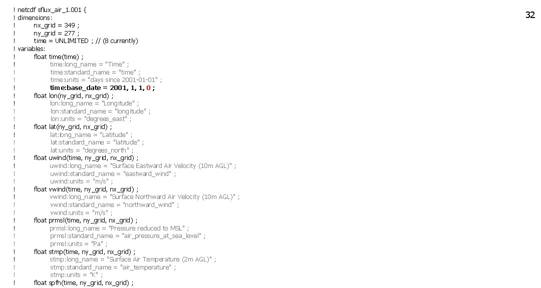
! netcdf sflux_air_1. 001 { ! dimensions: ! nx_grid = 349 ; ! ny_grid = 277 ; ! time = UNLIMITED ; // (8 currently) ! variables: ! float time(time) ; ! time: long_name = "Time" ; ! time: standard_name = "time" ; ! time: units = "days since 2001 -01 -01" ; ! time: base_date = 2001, 1, 1, 0 ; ! float lon(ny_grid, nx_grid) ; ! lon: long_name = "Longitude" ; ! lon: standard_name = "longitude" ; ! lon: units = "degrees_east" ; ! float lat(ny_grid, nx_grid) ; ! lat: long_name = "Latitude" ; ! lat: standard_name = "latitude" ; ! lat: units = "degrees_north" ; ! float uwind(time, ny_grid, nx_grid) ; ! uwind: long_name = "Surface Eastward Air Velocity (10 m AGL)" ; ! uwind: standard_name = "eastward_wind" ; ! uwind: units = "m/s" ; ! float vwind(time, ny_grid, nx_grid) ; ! vwind: long_name = "Surface Northward Air Velocity (10 m AGL)" ; ! vwind: standard_name = "northward_wind" ; ! vwind: units = "m/s" ; ! float prmsl(time, ny_grid, nx_grid) ; ! prmsl: long_name = "Pressure reduced to MSL" ; ! prmsl: standard_name = "air_pressure_at_sea_level" ; ! prmsl: units = "Pa" ; ! float stmp(time, ny_grid, nx_grid) ; ! stmp: long_name = "Surface Air Temperature (2 m AGL)" ; ! stmp: standard_name = "air_temperature" ; ! stmp: units = "K" ; ! float spfh(time, ny_grid, nx_grid) ; 32

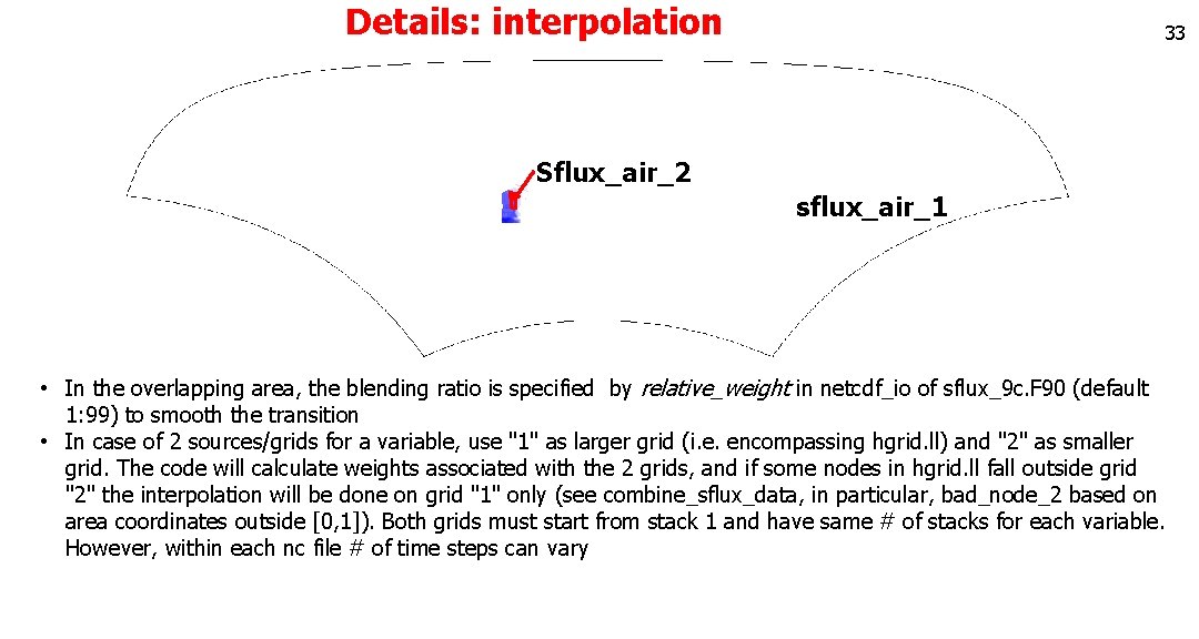
Details: interpolation 33 Sflux_air_2 sflux_air_1 • In the overlapping area, the blending ratio is specified by relative_weight in netcdf_io of sflux_9 c. F 90 (default 1: 99) to smooth the transition • In case of 2 sources/grids for a variable, use "1" as larger grid (i. e. encompassing hgrid. ll) and "2" as smaller grid. The code will calculate weights associated with the 2 grids, and if some nodes in hgrid. ll fall outside grid "2" the interpolation will be done on grid "1" only (see combine_sflux_data, in particular, bad_node_2 based on area coordinates outside [0, 1]). Both grids must start from stack 1 and have same # of stacks for each variable. However, within each nc file # of time steps can vary

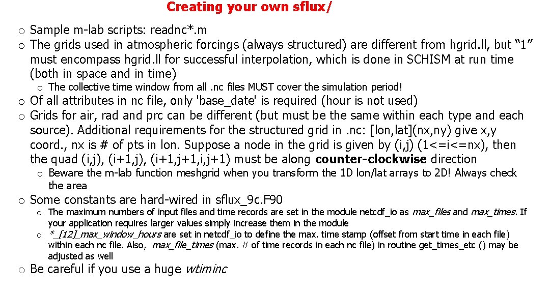
Creating your own sflux/ o Sample m-lab scripts: readnc*. m o The grids used in atmospheric forcings (always structured) are different from hgrid. ll, but “ 1” must encompass hgrid. ll for successful interpolation, which is done in SCHISM at run time (both in space and in time) o The collective time window from all. nc files MUST cover the simulation period! o Of all attributes in nc file, only 'base_date' is required (hour is not used) o Grids for air, rad and prc can be different (but must be the same within each type and each source). Additional requirements for the structured grid in. nc: [lon, lat](nx, ny) give x, y coord. , nx is # of pts in lon. Suppose a node in the grid is given by (i, j) (1<=i<=nx), then the quad (i, j), (i+1, j+1, i, j+1) must be along counter-clockwise direction o Beware the m-lab function meshgrid when you transform the 1 D lon/lat arrays to 2 D! Always check the area o Some constants are hard-wired in sflux_9 c. F 90 o The maximum numbers of input files and time records are set in the module netcdf_io as max_files and max_times. If your application requires larger values simply increase them in the module o *_[12]_max_window_hours are set in netcdf_io to define the max. time stamp (offset from start time in each file) within each nc file. Also, max_file_times (max. # of time records in each nc file) in routine get_times_etc () may be adjusted as well o Be careful if you use a huge wtiminc

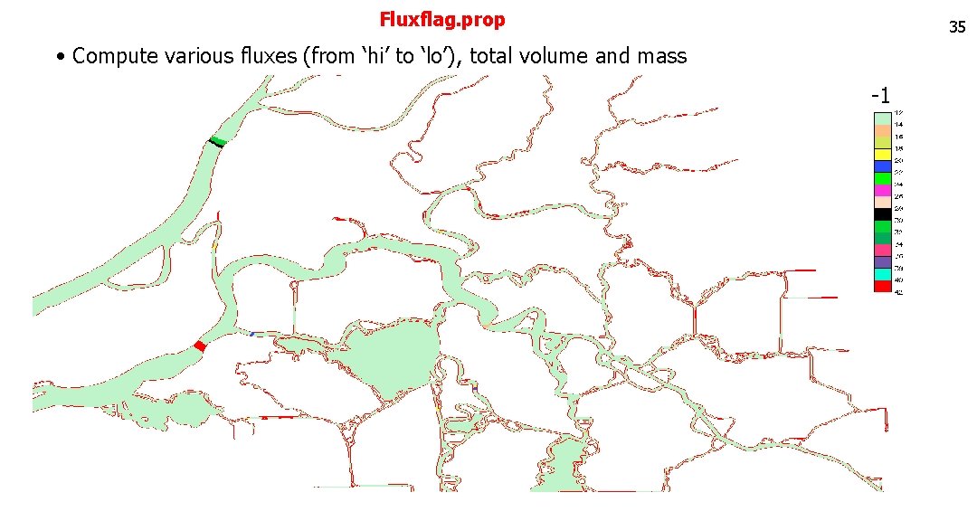
Fluxflag. prop 35 • Compute various fluxes (from ‘hi’ to ‘lo’), total volume and mass -1

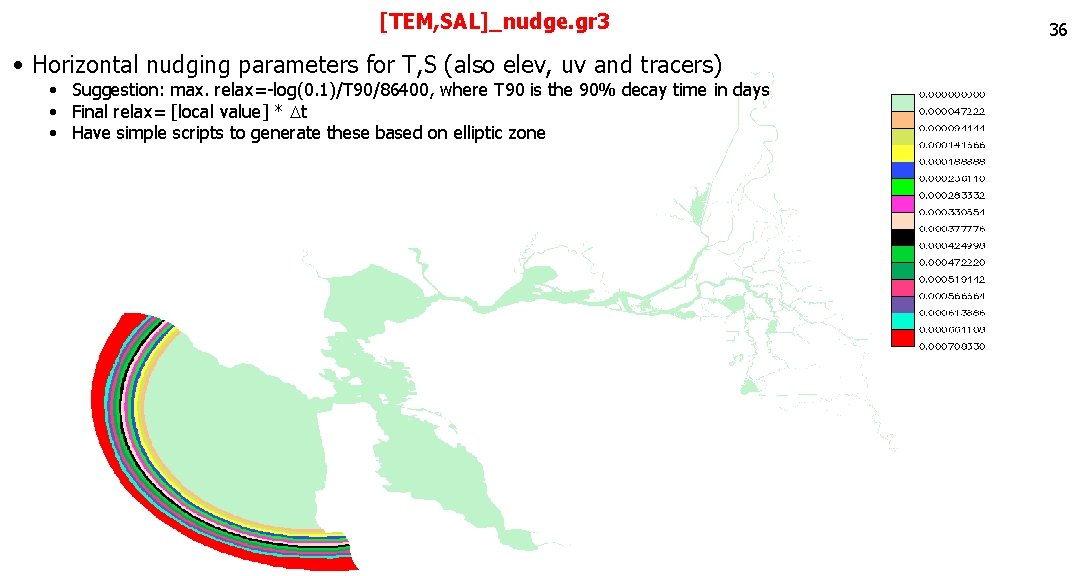
[TEM, SAL]_nudge. gr 3 • Horizontal nudging parameters for T, S (also elev, uv and tracers) • Suggestion: max. relax=-log(0. 1)/T 90/86400, where T 90 is the 90% decay time in days • Final relax= [local value] * Dt • Have simple scripts to generate these based on elliptic zone 36

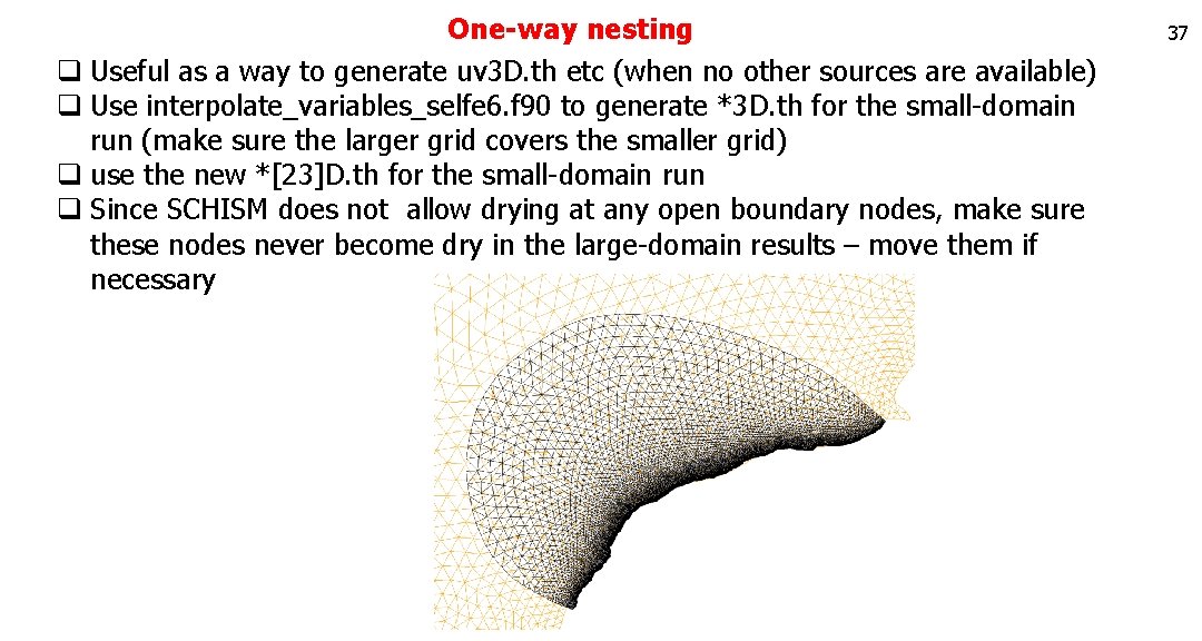
One-way nesting q Useful as a way to generate uv 3 D. th etc (when no other sources are available) q Use interpolate_variables_selfe 6. f 90 to generate *3 D. th for the small-domain run (make sure the larger grid covers the smaller grid) q use the new *[23]D. th for the small-domain run q Since SCHISM does not allow drying at any open boundary nodes, make sure these nodes never become dry in the large-domain results – move them if necessary 37

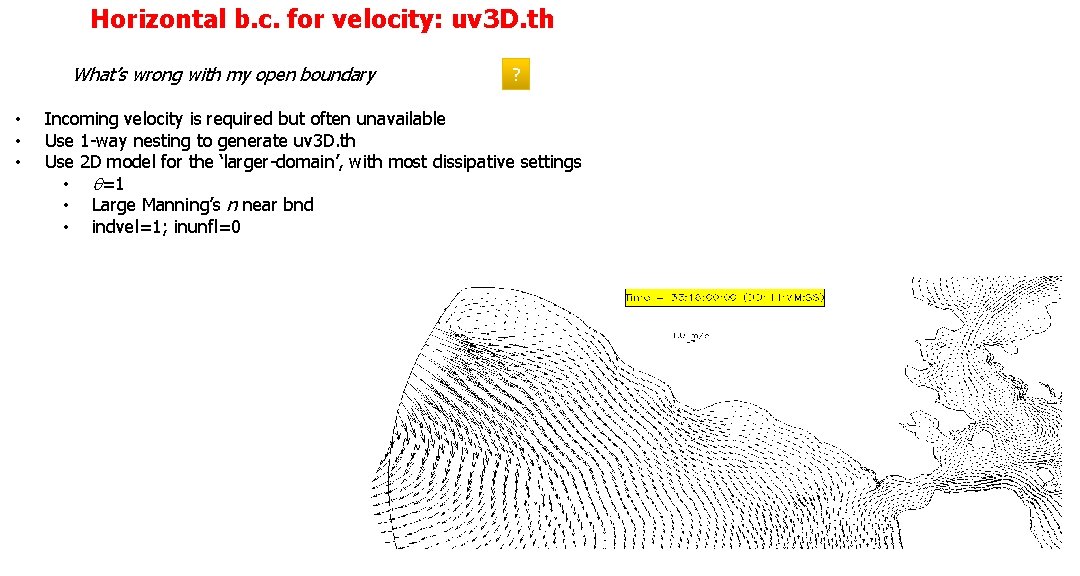
Horizontal b. c. for velocity: uv 3 D. th What’s wrong with my open boundary • • • ? Incoming velocity is required but often unavailable Use 1 -way nesting to generate uv 3 D. th Use 2 D model for the ‘larger-domain’, with most dissipative settings • q=1 • Large Manning’s n near bnd • indvel=1; inunfl=0

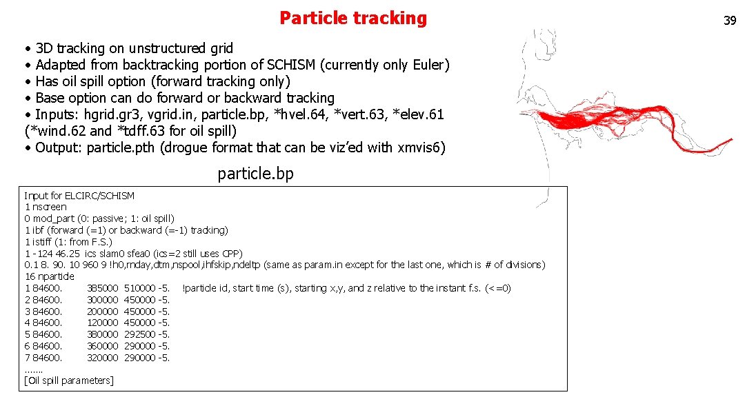
Particle tracking • 3 D tracking on unstructured grid • Adapted from backtracking portion of SCHISM (currently only Euler) • Has oil spill option (forward tracking only) • Base option can do forward or backward tracking • Inputs: hgrid. gr 3, vgrid. in, particle. bp, *hvel. 64, *vert. 63, *elev. 61 (*wind. 62 and *tdff. 63 for oil spill) • Output: particle. pth (drogue format that can be viz’ed with xmvis 6) particle. bp Input for ELCIRC/SCHISM 1 nscreen 0 mod_part (0: passive; 1: oil spill) 1 ibf (forward (=1) or backward (=-1) tracking) 1 istiff (1: from F. S. ) 1 -124 46. 25 ics slam 0 sfea 0 (ics=2 still uses CPP) 0. 1 8. 90. 10 960 9 !h 0, rnday, dtm, nspool, ihfskip, ndeltp (same as param. in except for the last one, which is # of divisions) 16 nparticle 1 84600. 385000 510000 -5. !particle id, start time (s), starting x, y, and z relative to the instant f. s. (<=0) 2 84600. 300000 450000 -5. 3 84600. 200000 450000 -5. 4 84600. 120000 450000 -5. 5 84600. 380000 292500 -5. 6 84600. 360000 290000 -5. 7 84600. 320000 290000 -5. ……. [Oil spill parameters] 39

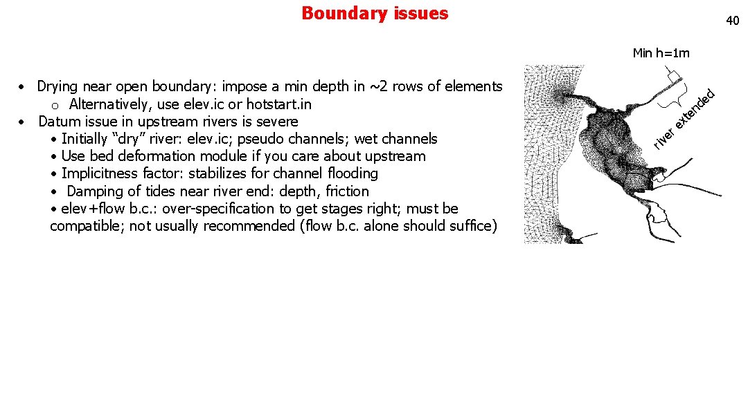
Boundary issues 40 Min h=1 m • Drying near open boundary: impose a min depth in ~2 rows of elements o Alternatively, use elev. ic or hotstart. in • Datum issue in upstream rivers is severe • Initially “dry” river: elev. ic; pseudo channels; wet channels • Use bed deformation module if you care about upstream • Implicitness factor: stabilizes for channel flooding • Damping of tides near river end: depth, friction • elev+flow b. c. : over-specification to get stages right; must be compatible; not usually recommended (flow b. c. alone should suffice) d en t ex ri r e v

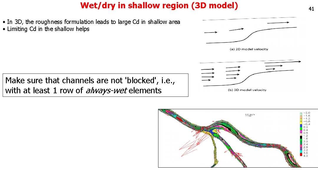
Wet/dry in shallow region (3 D model) • In 3 D, the roughness formulation leads to large Cd in shallow area • Limiting Cd in the shallow helps Make sure that channels are not 'blocked', i. e. , with at least 1 row of always-wet elements 41

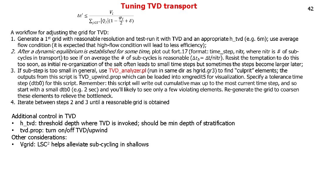
Tuning TVD transport Additional control in TVD • h_tvd: threshold depth where TVD is invoked; should be min depth of stratification • tvd. prop: turn on/off TVD/upwind Other considerations: • Vgrid: LSC 2 helps alleviate sub-cycling in shallows 42

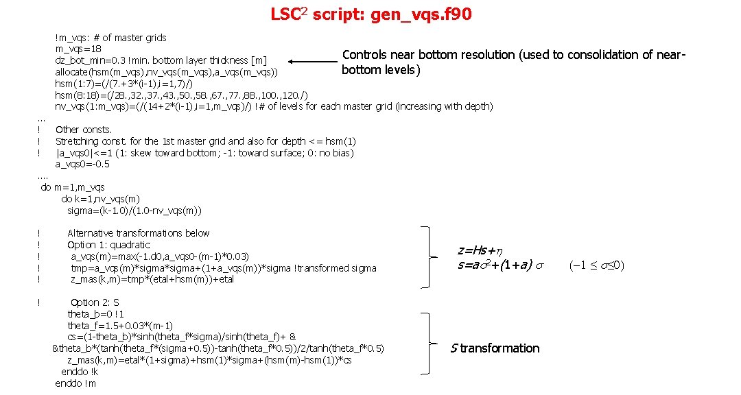
LSC 2 script: gen_vqs. f 90 !m_vqs: # of master grids m_vqs=18 Controls near bottom resolution (used to consolidation of near dz_bot_min=0. 3 !min. bottom layer thickness [m] bottom levels) allocate(hsm(m_vqs), nv_vqs(m_vqs), a_vqs(m_vqs)) hsm(1: 7)=(/(7. +3*(i-1), i=1, 7)/) hsm(8: 18)=(/28. , 32. , 37. , 43. , 50. , 58. , 67. , 77. , 88. , 100. , 120. /) nv_vqs(1: m_vqs)=(/(14+2*(i-1), i=1, m_vqs)/) !# of levels for each master grid (increasing with depth) … ! Other consts. ! Stretching const. for the 1 st master grid and also for depth <= hsm(1) ! |a_vqs 0|<=1 (1: skew toward bottom; -1: toward surface; 0: no bias) a_vqs 0=-0. 5 …. do m=1, m_vqs do k=1, nv_vqs(m) sigma=(k-1. 0)/(1. 0 -nv_vqs(m)) ! Alternative transformations below ! Option 1: quadratic ! a_vqs(m)=max(-1. d 0, a_vqs 0 -(m-1)*0. 03) ! tmp=a_vqs(m)*sigma+(1+a_vqs(m))*sigma !transformed sigma ! z_mas(k, m)=tmp*(etal+hsm(m))+etal ! Option 2: S theta_b=0 !1 theta_f=1. 5+0. 03*(m-1) cs=(1 -theta_b)*sinh(theta_f*sigma)/sinh(theta_f)+ & &theta_b*(tanh(theta_f*(sigma+0. 5))-tanh(theta_f*0. 5))/2/tanh(theta_f*0. 5) z_mas(k, m)=etal*(1+sigma)+hsm(1)*sigma+(hsm(m)-hsm(1))*cs enddo !k enddo !m z=Hs+h s=as 2+(1+a) s S transformation (-1 ≤ s≤ 0)

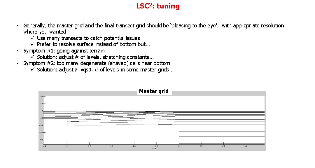
LSC 2: tuning • Generally, the master grid and the final transect grid should be ‘pleasing to the eye’, with appropriate resolution where you wanted ü Use many transects to catch potential issues ü Prefer to resolve surface instead of bottom but… • Symptom #1: going against terrain ü Solution: adjust # of levels, stretching constants… • Symptom #2: too many degenerate (shaved) cells near bottom ü Solution: adjust a_vqs 0, # of levels in some master grids… Master grid

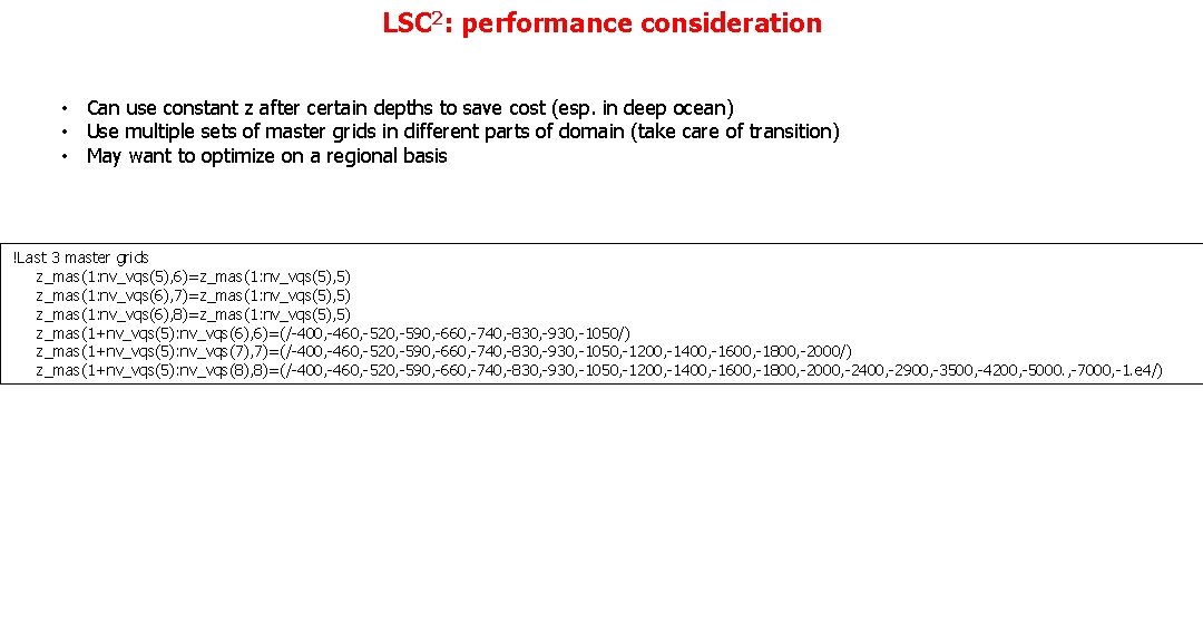
LSC 2: performance consideration • Can use constant z after certain depths to save cost (esp. in deep ocean) • Use multiple sets of master grids in different parts of domain (take care of transition) • May want to optimize on a regional basis !Last 3 master grids z_mas(1: nv_vqs(5), 6)=z_mas(1: nv_vqs(5), 5) z_mas(1: nv_vqs(6), 7)=z_mas(1: nv_vqs(5), 5) z_mas(1: nv_vqs(6), 8)=z_mas(1: nv_vqs(5), 5) z_mas(1+nv_vqs(5): nv_vqs(6), 6)=(/-400, -460, -520, -590, -660, -740, -830, -930, -1050/) z_mas(1+nv_vqs(5): nv_vqs(7), 7)=(/-400, -460, -520, -590, -660, -740, -830, -930, -1050, -1200, -1400, -1600, -1800, -2000/) z_mas(1+nv_vqs(5): nv_vqs(8), 8)=(/-400, -460, -520, -590, -660, -740, -830, -930, -1050, -1200, -1400, -1600, -1800, -2000, -2400, -2900, -3500, -4200, -5000. , -7000, -1. e 4/)