Using rasterbased timeseries analysis to define temporal streamflow

Using raster-based time-series analysis to define temporal streamflow variability; Keeping the ‘natural’ in natural streamflow Richard Koehler, Ph. D. National Weather Service, NOAA

Quote: “There’s a saying among prospectors: ‘Go out looking for one thing, and that’s all you’ll ever find. ’ ” Robert Flaherty (1884 – 1951) legendary documentary filmmaker

Presentation outline Study sites n Background n Theoretical overview n Raster-based image n Grid-correlograms n Patch analysis n Results n Other applications n Questions n

Study sites n Snake and Colorado Rivers n Snowmelt runoff dominated n Highly regulated n Tributaries with minimal human disturbances n San Pedro River n Rainfall dominated n Unregulated

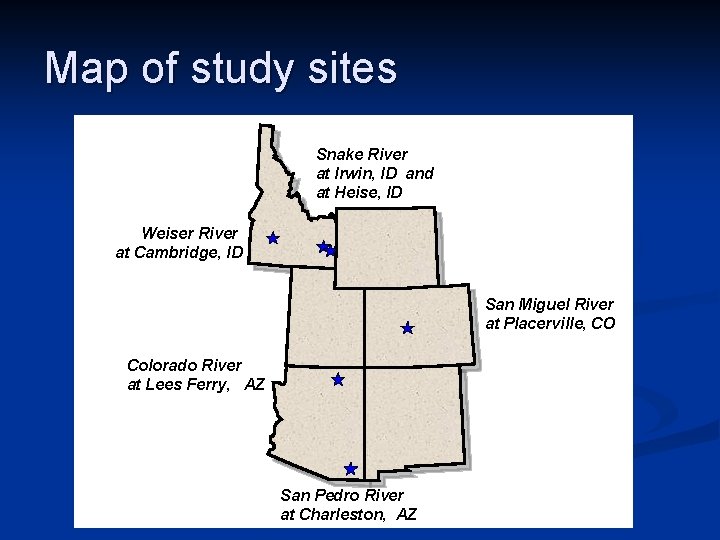
Map of study sites Snake River at Irwin, ID and at Heise, ID Weiser River at Cambridge, ID San Miguel River at Placerville, CO Colorado River at Lees Ferry, AZ San Pedro River at Charleston, AZ

Background n Streamflow patterns n n Multiple existing methods (170+ indices ) n n Occur on different timescales Show cumulative effect of disturbances Include flow volume and timing Many correlated or redundant Adequate for volume (composition) Weak for timing (configuration) Large daily datasets exist n Possibility for many types of patterns within flow record

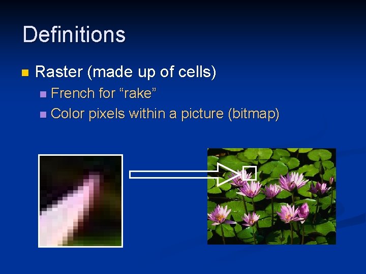
Definitions n Raster (made up of cells) French for “rake” n Color pixels within a picture (bitmap) n

Arecibo Message example n Binary message Radio astronomy message transmitted in 1974 n Repeating 1, 679 bit length (23 x 73) n n Information through adjacency 0010001110101100000 Part of the binary Arecibo Message

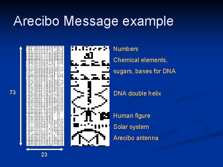
Arecibo Message example Numbers Chemical elements, sugars, bases for DNA 73 DNA double helix Human figure Solar system Arecibo antenna 23

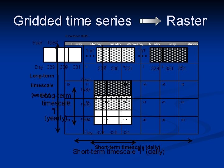
Gridded time series Raster November 1985 Year 1984 Sunday 1985 Tuesday Monday Wednesday . . . 1 yr Day 329 3303 Long-term timescale 331 4 1986 Thursday 3295 330 Friday 1 2 6 7 12 13 14 15 16 19 20 21 22 23 26 27 28 29 30 331 329 8 Saturday 330 9 331 Year 10 (weekly) Long-term 17 timescale "j" (yearly)24 11 1986 18 1985 1984 25 Day 329 330 331 Short-term timescale (daily) Short-term timescale "i" (daily)

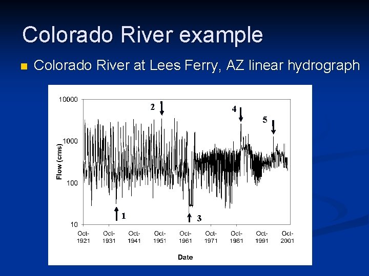
Colorado River example n Colorado River at Lees Ferry, AZ linear hydrograph 2 4 5 1 3

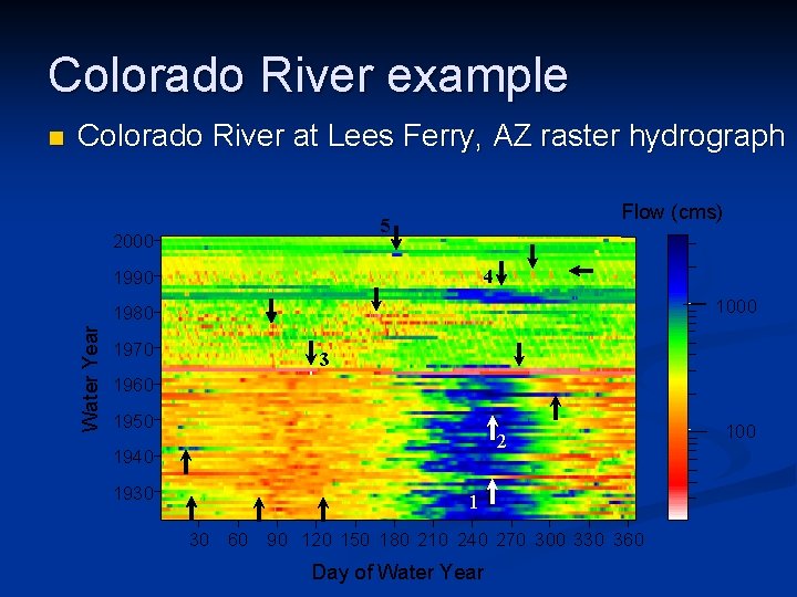
Colorado River example Colorado River at Lees Ferry, AZ raster hydrograph Flow (cms) 5 2000 4 1990 1980 Water Year n 1970 3. 00 1000 3 1960 1950 2 1940 1930 1 30 60 90 120 150 180 210 240 270 300 330 360 Day of Water Year 2. 00 100

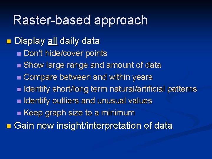
Raster-based approach n Display all daily data Don’t hide/cover points n Show large range and amount of data n Compare between and within years n Identify short/long term natural/artificial patterns n Identify outliers and unusual values n Keep graph size to a minimum n n Gain new insight/interpretation of data

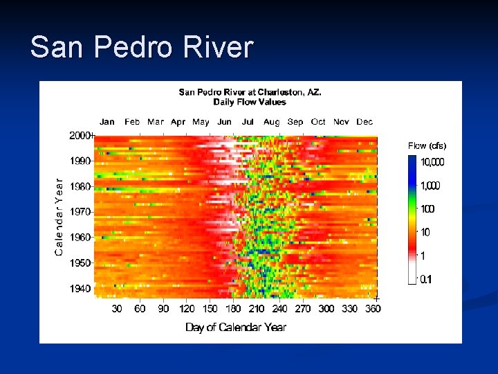
San Pedro River + +

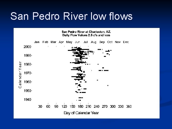
San Pedro River low flows

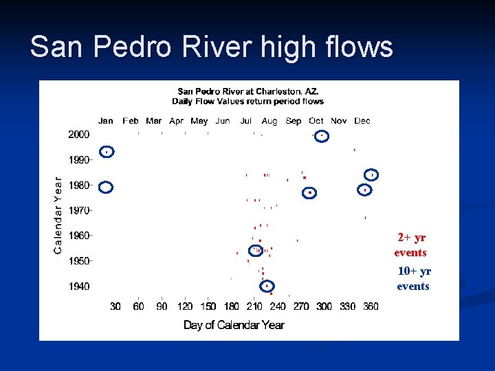
San Pedro River high flows 2+ yr events 10+ yr events

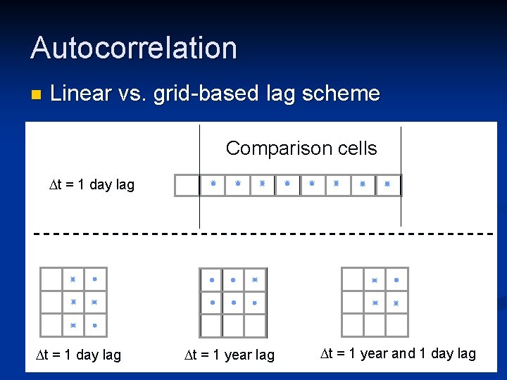
Autocorrelation n Linear vs. grid-based lag scheme Comparison cells Dt = 1 day lag Dt = 1 year and 1 day lag

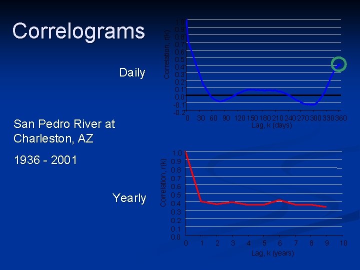
Daily Correlation, r(k) Correlograms 1. 0 0. 9 0. 8 0. 7 0. 6 0. 5 0. 4 0. 3 0. 2 0. 1 0. 0 -0. 1 -0. 2 1936 - 2001 Yearly Correlation, r(k) San Pedro River at Charleston, AZ 1. 0 0. 9 0. 8 0. 7 0. 6 0. 5 0. 4 0. 3 0. 2 0. 1 0. 0 0 0 30 60 90 120 150 180 210 240 270 300 330 360 Lag, k (days) 1 2 3 4 5 6 7 Lag, k (years) 8 9 10

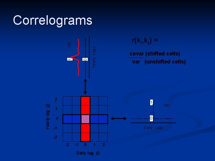
Correlograms Yearly Lags 0 1 r(k) r(ki, kj) = covar (shifted cells) var (unshifted cells) Yearly lag (j) 2 1 1 0 0 Daily Lags -1 -2 -2 -1 0 1 Daily lag (i) 2 r(k)

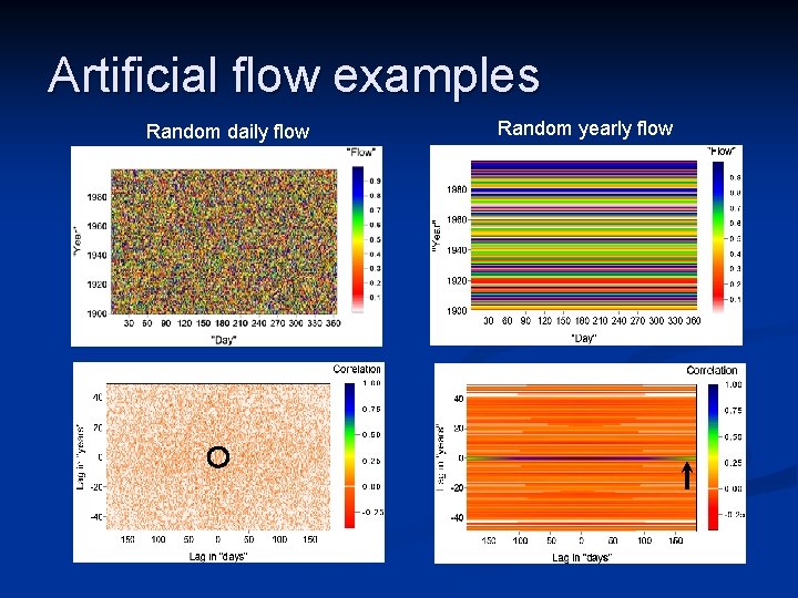
Artificial flow examples Random daily flow Random yearly flow

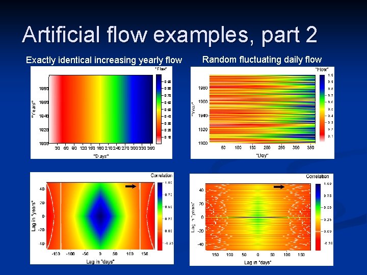
Artificial flow examples, part 2 Exactly identical increasing yearly flow "Flow" 0. 90 1980 0. 80 "Years" 0. 70 1960 0. 50 1940 0. 30 1920 0. 10 1900 30 60 90 120 150 180 210 240 270 300 330 360 "Days" Random fluctuating daily flow

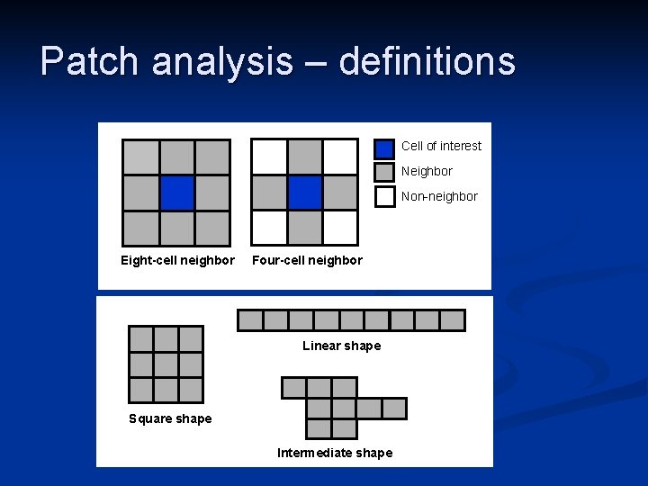
Patch analysis – definitions Cell of interest Neighbor Non-neighbor Eight-cell neighbor Four-cell neighbor Linear shape Square shape Intermediate shape

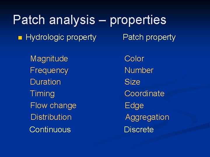
Patch analysis – properties n Hydrologic property Magnitude Frequency Duration Timing Flow change Distribution Continuous Patch property Color Number Size Coordinate Edge Aggregation Discrete

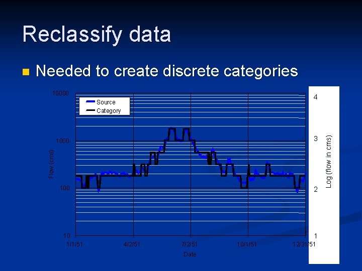
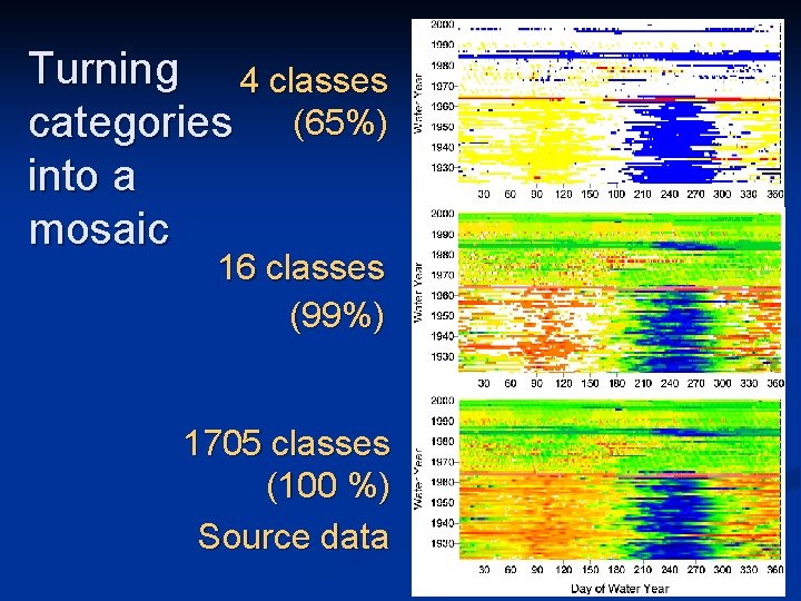
Reclassify data Needed to create discrete categories 10000 1000 3 100 2 10 1/1/51 1 4/2/51 7/2/51 Date 10/1/51 12/31/51 Log (flow in cms) 4 Source Category Flow (cms) n

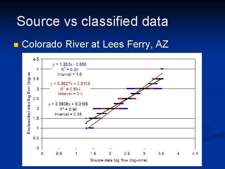
Source vs classified data n Colorado River at Lees Ferry, AZ

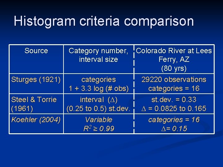
Histogram criteria comparison Source Category number, Colorado River at Lees interval size Ferry, AZ (80 yrs) Sturges (1921) categories 29220 observations 1 + 3. 3 log (# obs) categories = 16 Steel & Torrie interval (D) st. dev. = 0. 33 (1961) (0. 25 to 0. 5) st. dev. D = 0. 0825 to 0. 165 Koehler (2004) Variable categories = 16 R 2 ≥ 0. 99 D= 0. 15

Turning 4 classes categories (65%) into a mosaic 16 classes (99%) 1705 classes (100 %) Source data

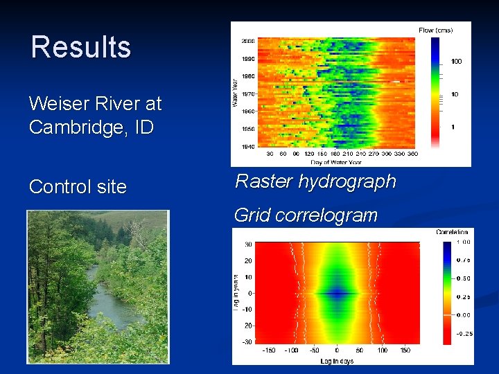
Results Weiser River at Cambridge, ID Control site Raster hydrograph Grid correlogram

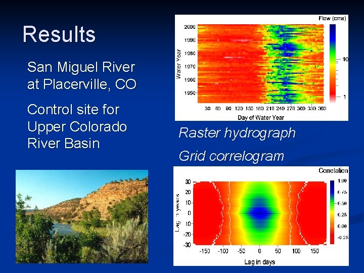
Results San Miguel River at Placerville, CO Control site for Upper Colorado River Basin Raster hydrograph Grid correlogram

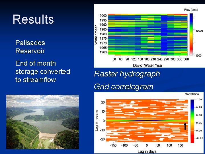
Results Palisades Reservoir End of month storage converted to streamflow Raster hydrograph Grid correlogram

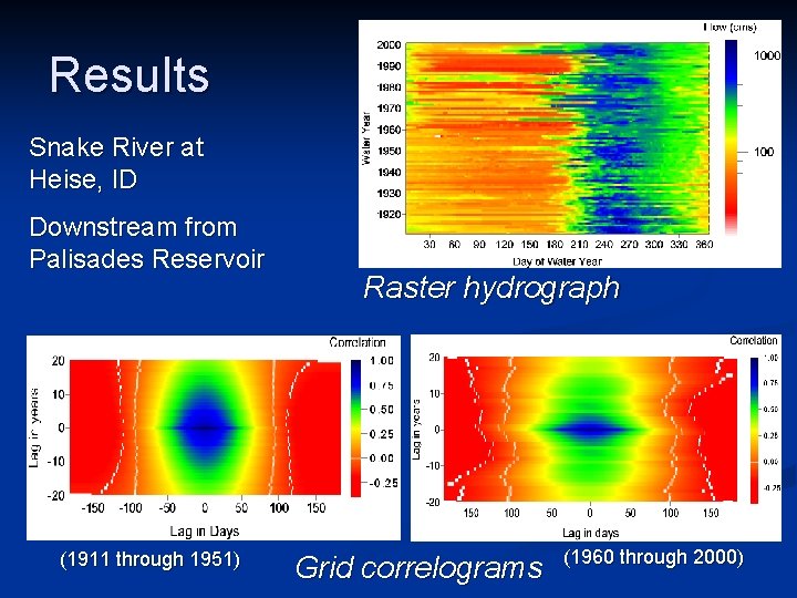
Results Snake River at Heise, ID Downstream from Palisades Reservoir (1911 through 1951) Raster hydrograph Grid correlograms (1960 through 2000)

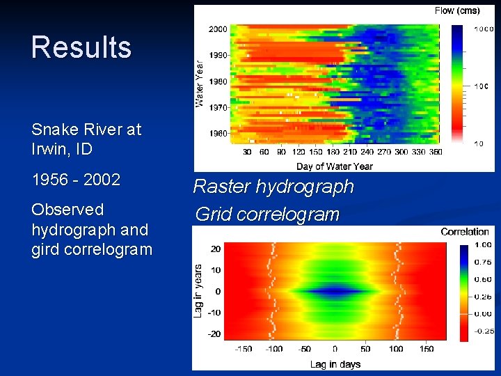
Results Snake River at Irwin, ID 1956 - 2002 Observed hydrograph and gird correlogram Raster hydrograph Grid correlogram

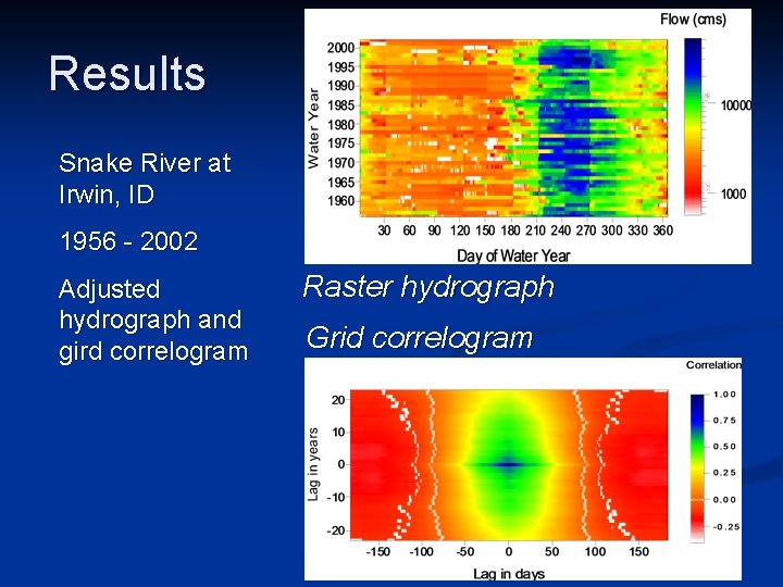
Results Snake River at Irwin, ID 1956 - 2002 Adjusted hydrograph and gird correlogram Raster hydrograph Grid correlogram

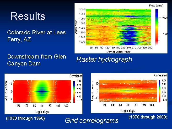
Results Colorado River at Lees Ferry, AZ Downstream from Glen Canyon Dam (1930 through 1960) Raster hydrograph Grid correlograms (1970 through 2000)

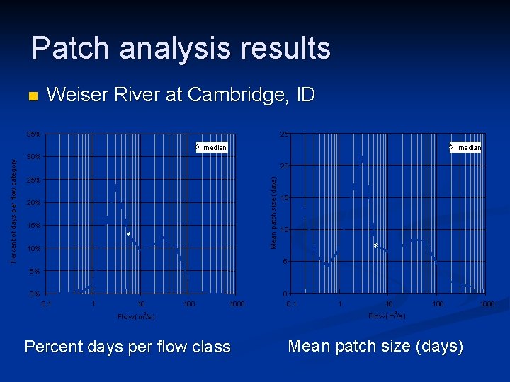
Patch analysis results n Weiser River at Cambridge, ID 25 35% median 20 25% Mean patch size (days) Percent of days per flow category median 30% 20% 15% 10% 15 10 5 5% 0% 0. 1 1 10 1000 3 Flow (m /s) Percent days per flow class 0 0. 1 1 10 100 3 Flow (m /s) Mean patch size (days) 1000

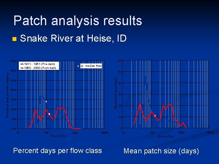
Patch analysis results 35% Percent of days per flow category 30% Snake River at Heise, ID 60 1911 - 1951 (Pre-dam) 1960 - 2000 (Post-dam) median flow 50 Mean patch area (days) n 25% 20% 15% 10% 40 30 20 10 5% 0 0% 10 100 3 Flow (m /s) 10000 Percent days per flow class 10 100 3 1000 Flow (m /s) Mean patch size (days) 10000

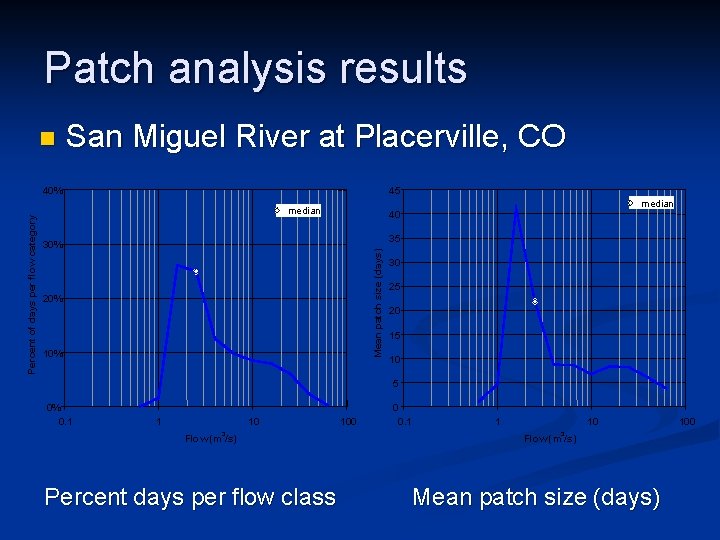
Patch analysis results n San Miguel River at Placerville, CO 45 median 40 35 30% Mean patch size (days) Percent of days per flow category 40% 20% 10% 30 25 20 15 10 5 0% 0. 1 1 10 3 Flow (m /s) Percent days per flow class 100 0 0. 1 1 10 3 Flow (m /s) Mean patch size (days) 100

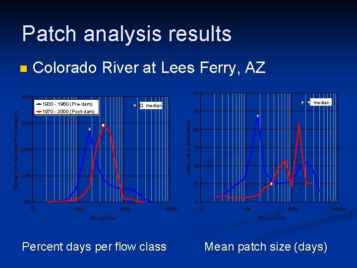
Patch analysis results n Colorado River at Lees Ferry, AZ 30 40% median 25 1970 - 2000 (Post-dam) Mean patch size (days) Percent of days per flow category 1930 - 1960 (Pre-dam) 30% 20% 10% 20 15 10 5 0% 10 0 10000 3 Flow (m /s) Percent days per flow class 10 1000 3 Flow (m /s) Mean patch size (days) 10000

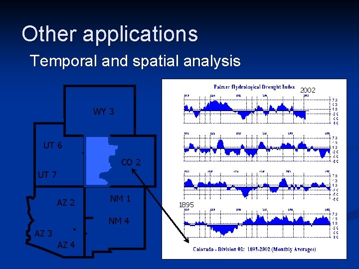
Other applications Temporal and spatial analysis 2002 WY 3 UT 6 CO 2 UT 7 AZ 2 NM 1 NM 4 AZ 3 AZ 4 1895

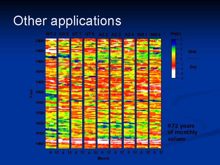
Other applications WY 3 CO 2 UT 7 UT 6 AZ 2 AZ 3 AZ 4 NM 1 NM 4 Year 2000 2000 2000 1990 1990 1980 1980 1970 1970 1960 1960 1950 1950 1940 1940 1930 1930 1920 1920 1910 1910 1900 1900 6 12 6 12 1900 6 12 Month PHDI 8 6 4 2 0 -2 -4 -6 -8 Wet Dry 972 years of monthly values 6 12

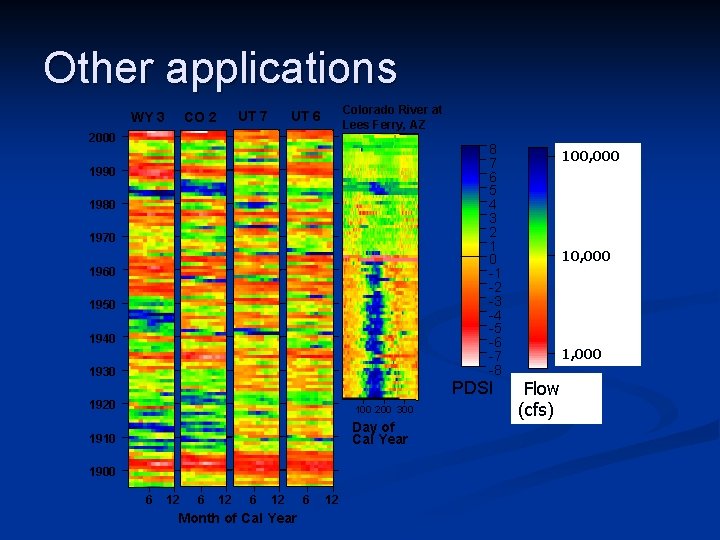
Other applications WY 3 2000 UT 7 CO 2 2000 1990 1980 1970 1960 1950 1940 1930 1920 1910 1900 Colorado River at Lees Ferry, AZ UT 6 8 7 6 5 4 3 2 1 0 -1 -2 -3 -4 -5 -6 -7 -8 PDSI 1900 6 12 Month of Cal Year 100 200 300 Day of Cal Year 6 12 100, 000 1, 000 Flow (cfs)

Summary Traditional methods limited n Raster-based approach n n Greater visualization n Raster n hydrograph New tools to analyze streamflow n Grid correlogram n Patch analysis n Numerous applications / research directions New approach to identify temporal variability n Enhance and replicate streamflow conditions n

Questions?