Using Multivariate Time Series Forecasting Models for Enrollment

Using Multivariate Time Series Forecasting Models for Enrollment Predictions Deirdre Syms, George Xia Macomb Community College November 5, 2015

Bring the Case into Statistical Analysis and Forecasting l A very interesting Macomb Community degree credit side student enrollment pattern over decades matches the local economic situation: – When the local economy turns better, the enrollment figure went down – When the local economy turns worse, the enrollment figure went up l As a typical suburban two-year college, we provide quality education with lower costs to our students, thus we assume local economic data such as unemployment rates are affect our students’ enrollment behaviors. l We/I do a lot of student enrollment reports at MCC, including each semester’s internal enrollment report, each middle fall’s IPEDS enrollment report, etc. Almost all these reports focus on the data facts and descriptive statistics. They are not related to inferential statistical analysis. l Today, there a lot of statistical analysis and forecasting tools for us to use in this case if we want to dig more useful information from our enrollment data, especially predicting the near future student enrollment. The tools may includes the recent versions of SAS/ETS and SPSS.

Pre-Data Analysis Considerations l l l Before every inferential statistical analysis with modeling building, we have to examine if our statistical model(s) chosen is appropriate to our case. For example, in the most common analysis using ordinary two -sample t-test, each observation of data has to meet with three assumptions: independent each other, statistically identical variation, and normally distributed. To qualify a series of data to use statistical software such as SAS/ETS, the time series data need assumptions such as: – – – Data points gathered sequentially through equal time periods Future value depends upon the present value and the present value depends on the past observations, the series length is 30 or more Stochastically stationary or can be mathematically converted into stationary

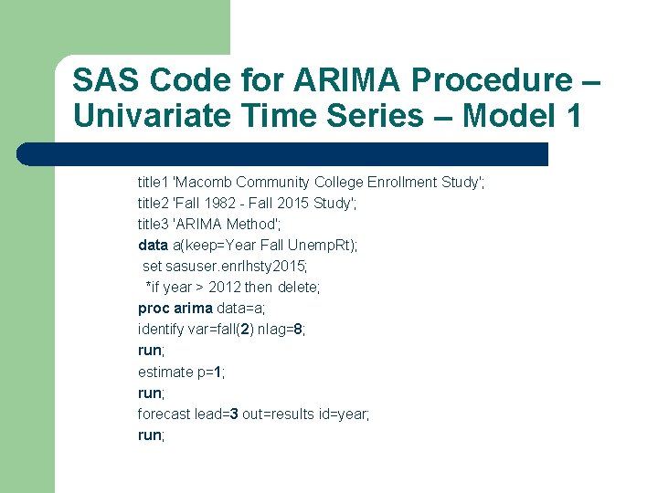
SAS/ETS Proc ARIMA Data Analysis – Univariate Time Series – Model 1 l Proc ARIMA, what does ARIMA mean? It means: A procedure of Auto Regressive Integrative Moving Average l There are three stages to proc ARIMA: – – – l Identification stage: to determine the degree of difference, d; also can use “nlag” to set up number of lags for autocorrelations are shown Estimation and diagnostic checking stage: to determine degree of auto regression, p; and degree of moving average, q; Forecasting stage: set up number of periods need to be predicted Thus ARIMA has three important parameters: ARIMA (p, d, q). In our case, after back and forth checking, we picked p = 1, nlag = 8 d = 2, and q = 0, i. e. , we have ARIMA (1, 2, 0) model, and we set up our forecast periods as 3.

SAS Code for ARIMA Procedure – Univariate Time Series – Model 1 title 1 'Macomb Community College Enrollment Study'; title 2 'Fall 1982 - Fall 2015 Study'; title 3 'ARIMA Method'; data a(keep=Year Fall Unemp. Rt); set sasuser. enrlhsty 2015; *if year > 2012 then delete; proc arima data=a; identify var=fall(2) nlag=8; run; estimate p=1; run; forecast lead=3 out=results id=year; run;

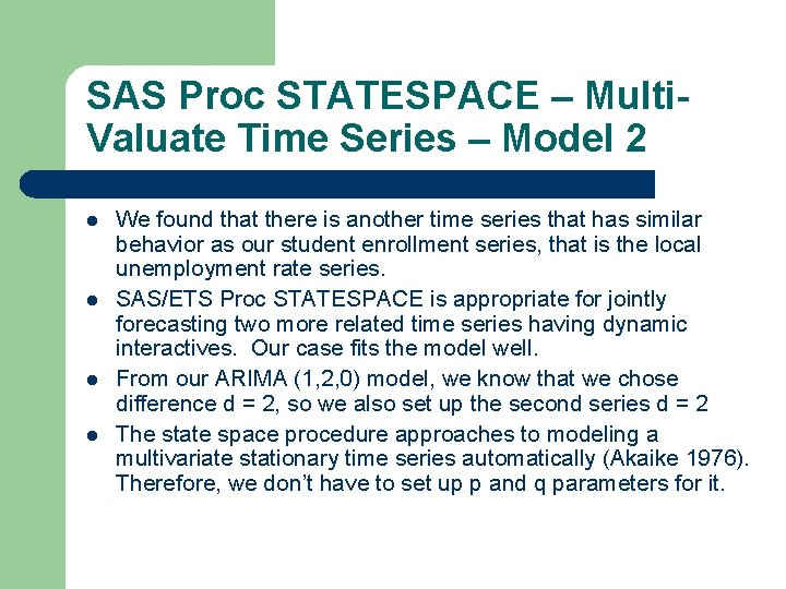
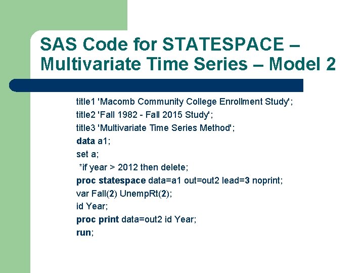
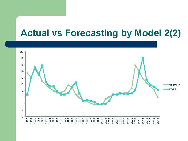
SAS Proc STATESPACE – Multi. Valuate Time Series – Model 2 l l We found that there is another time series that has similar behavior as our student enrollment series, that is the local unemployment rate series. SAS/ETS Proc STATESPACE is appropriate for jointly forecasting two more related time series having dynamic interactives. Our case fits the model well. From our ARIMA (1, 2, 0) model, we know that we chose difference d = 2, so we also set up the second series d = 2 The state space procedure approaches to modeling a multivariate stationary time series automatically (Akaike 1976). Therefore, we don’t have to set up p and q parameters for it.

SAS Code for STATESPACE – Multivariate Time Series – Model 2 title 1 'Macomb Community College Enrollment Study'; title 2 'Fall 1982 - Fall 2015 Study'; title 3 'Multivariate Time Series Method'; data a 1; set a; *if year > 2012 then delete; proc statespace data=a 1 out=out 2 lead=3 noprint; var Fall(2) Unemp. Rt(2); id Year; proc print data=out 2 id Year; run;

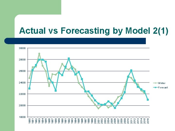
18000 1981 1982 1983 1984 1985 1986 1987 1988 1989 1990 1991 1992 1993 1994 1995 1996 1997 1998 1999 2000 2001 2002 2003 2004 2005 2006 2007 2008 2009 2010 2011 2012 2013 2014 2015 2016 Actual vs Forecasting by Model 2(1) 30000 28000 26000 24000 Winter Forecast 220000

0 1981 1982 1983 1984 1985 1986 1987 1988 1989 1990 1991 1992 1993 1994 1995 1996 1997 1998 1999 2000 2001 2002 2003 2004 2005 2006 2007 2008 2009 2010 2011 2012 2013 2014 2015 Actual vs Forecasting by Model 2(2) 20 18 16 14 12 10 Unemp. Rt 8 FOR 2 6 4 2

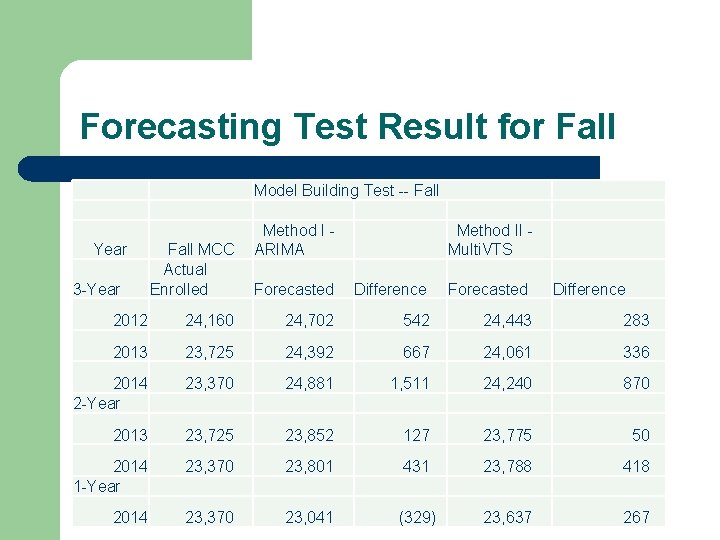
Forecasting Test Result for Fall Model Building Test -- Fall Year 3 -Year Fall MCC Actual Enrolled Method I ARIMA Method II Multi. VTS Forecasted Difference 2012 24, 160 24, 702 542 24, 443 283 2013 23, 725 24, 392 667 24, 061 336 2014 2 -Year 23, 370 24, 881 1, 511 24, 240 870 2013 23, 725 23, 852 127 23, 775 50 2014 1 -Year 23, 370 23, 801 431 23, 788 418 2014 23, 370 23, 041 (329) 23, 637 267

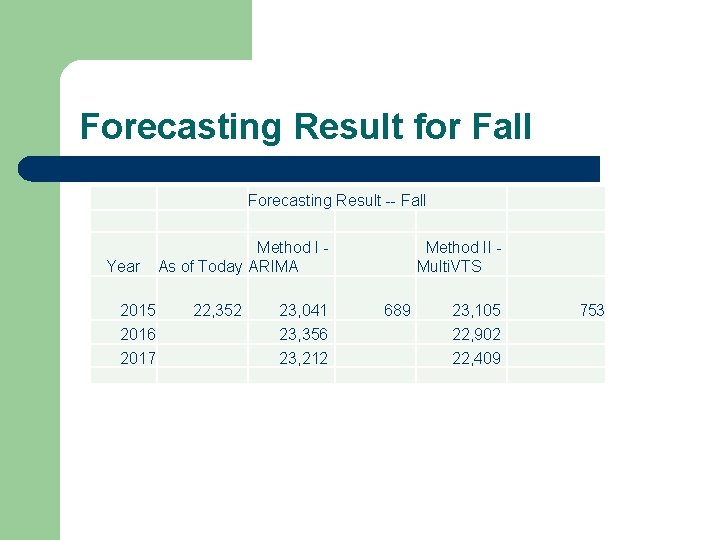
Forecasting Result for Fall Forecasting Result -- Fall Year 2015 2016 2017 Method I As of Today ARIMA 22, 352 23, 041 23, 356 23, 212 Method II Multi. VTS 689 23, 105 22, 902 22, 409 753

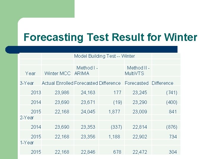
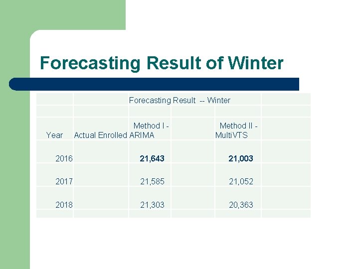
Forecasting Test Result for Winter Model Building Test -- Winter Year 3 -Year Method I Winter MCC ARIMA Method II Multi. VTS Actual Enrolled Forecasted Difference 2013 23, 986 24, 163 177 23, 245 (741) 2014 23, 690 23, 671 (19) 23, 290 (400) 2015 2 -Year 22, 168 24, 045 23, 009 841 2014 23, 690 23, 353 22, 814 (876) 2015 1 -Year 22, 168 23, 356 1, 188 22, 902 734 2015 22, 168 22, 846 678 22, 472 304 1, 877 (337)

Forecasting Result of Winter Forecasting Result -- Winter Year Method I Actual Enrolled ARIMA Method II Multi. VTS 2016 21, 643 21, 003 2017 21, 585 21, 052 2018 21, 303 20, 363

Research Notes l l l Two types of time series models we mentioned, a univariate one and a multivariate one, we can compare and judge which one is better. The other model such as using SAS Proc PDL (polynomial distributed lag) also can be used. Since enrollment forecasts are difficult to make in periods of irregular patterns when turning points are unexpected. Therefore, subjective forecasting should not be ruled out. Actually, if we integrate our administrative experience and quantitative analysis, the forecasting may more accurate. Some factors are important, such as marketing effort, improve our program and curriculum set up, teaching reputation, etc. , however, these factors are very hard to quantified and hard to bring in. Also, comparing with most of four-year colleges and universities, we charge lower tuition and fees, a small increase of tuition and fees will not affect enrollment much.

References l l SAS Institute (1993), SAS/ETS User’s Guide V 6 second Edition SAS Inc. Abraham, B. and Ledolter, J. (1983). Statistical Method for Forecasting Chen, C. (2008) Meharry Medical College, An Integrated Enrollment Forecast Model, IR Applications V. 15 Xia, Z. 2001, Macomb Community College Student Enrollment Model Building with Trend Analysis and Forecasting