Using Machine Learning Models to Predict Costs under

Using Machine Learning Models to Predict Costs under Alternative Designs in a Responsive Design Framework James Wagner 1, 2, Michael Elliott 1, 2, 3, Brady T. West 1, 2, Stephanie Coffey 2, 3 1 Survey Research Center, Institute for Social Research, Univ. of MIAnn Arbor 2 Joint Program in Survey Methodology, Univ. of MD-College Park 3 U. S. Census Bureau © 2019 by the Regents of the University of Michigan ESRA July 18, 2019

Acknowledgements / Disclaimers • This work was supported by a grant from the National Institutes for Health (#1 R 01 AG 058599‐ 01; PI: Wagner) • The National Survey of Family Growth (NSFG) is conducted by the Centers for Disease Control and Prevention's (CDC’s) National Center for Health Statistics (NCHS), under contract # 200‐ 2010‐ 33976 with University of Michigan’s Institute for Social Research with funding from several agencies of the U. S. Department of Health and Human Services, including CDC/NCHS, the National Institute of Child Health and Human Development (NICHD), the Office of Population Affairs (OPA), and others listed on the NSFG webpage (see http: //www. cdc. gov/nchs/nsfg/). The views expressed here do not represent those of NCHS or the other funding agencies. 2 © 2019 by the Regents of the University of Michigan

Overview • Background – Responsive Survey Design – Monitoring incoming data from the field • Problem – Need predictions of costs under alternative designs • NSFG – Current design – Data • Methods – Multilevel Regression Models – Bayesian Additive Regression Trees (BART) • Results • Conclusions 3 © 2019 by the Regents of the University of Michigan

Responsive Survey Design (RSD) • Uncertainty has become an issue in survey design • RSD makes use of incoming data from the field to address this uncertainty – Groves and Heeringa (2006) • Develop indicators of cost and error • Planned interventions when costs increase or errors stabilize/increase 4 © 2019 by the Regents of the University of Michigan

Problem • Costs and errors vary over time • RSD has used proxy indicators – Costs: call attempts – Nonresponse error: stabilized estimates, “phase capacity” • Inaccurate indicators may lead to inefficient designs • Can we improve the accuracy of cost predictions? 5 © 2019 by the Regents of the University of Michigan

NSFG • Continuous data collection – A new sample is released every quarter • Two‐stage data collection: – Screener interview to identify eligible persons – Main interview of selected person • Two phases of data collection: – Phase 1: 10 week data collection – Phase 2: Subsample remaining cases § Oversample higher likelihood of interview cases and eligible/likely eligible cases § Reduce interviewer workload by 2/3 § Change data collection model: added interview token of appreciation, interviewer behavior change – Combine data and response rates from two phases using weights 6 © 2019 by the Regents of the University of Michigan

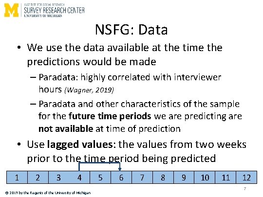
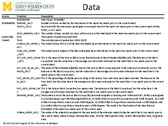
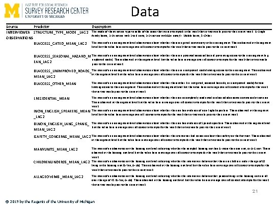
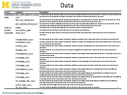
NSFG: Data • We use the data available at the time the predictions would be made – Paradata: highly correlated with interviewer hours (Wagner, 2019) – Paradata and other characteristics of the sample for the future time periods we are predicting are not available at time of prediction • Use lagged values: the values from two weeks prior to the time period being predicted © 2019 by the Regents of the University of Michigan 7

NSFG: Data • Data include: – Interviewer ID – Phase (i. e. the design change) – Lagged values of the following: • Area characteristics: Census Division, Population eligibility rate, urbanicity, etc. • Interviewer observations: access problems, safety concerns, etc. • Commercial data: Age of first person, etc. • Paradata: Number of screened interviews, number of trips, number of active lines, etc. © 2019 by the Regents of the University of Michigan 8

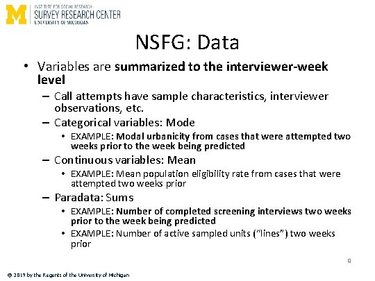
NSFG: Data • Variables are summarized to the interviewer-week level – Call attempts have sample characteristics, interviewer observations, etc. – Categorical variables: Mode • EXAMPLE: Modal urbanicity from cases that were attempted two weeks prior to the week being predicted – Continuous variables: Mean • EXAMPLE: Mean population eligibility rate from cases that were attempted two weeks prior – Paradata: Sums • EXAMPLE: Number of completed screening interviews two weeks prior to the week being predicted • EXAMPLE: Number of active sampled units (“lines”) two weeks prior 9 © 2019 by the Regents of the University of Michigan

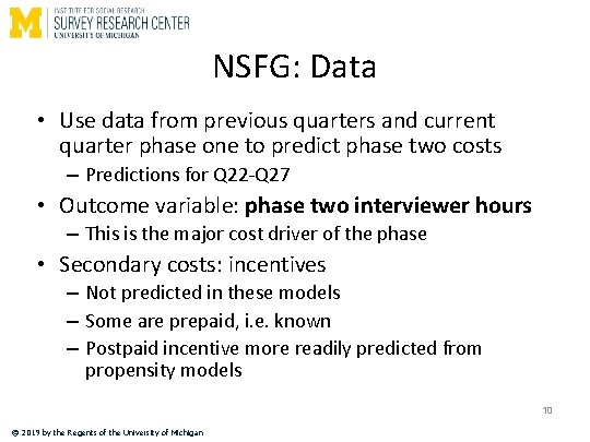
NSFG: Data • Use data from previous quarters and current quarter phase one to predict phase two costs – Predictions for Q 22‐Q 27 • Outcome variable: phase two interviewer hours – This is the major cost driver of the phase • Secondary costs: incentives – Not predicted in these models – Some are prepaid, i. e. known – Postpaid incentive more readily predicted from propensity models 10 © 2019 by the Regents of the University of Michigan

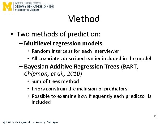
Method • Two methods of prediction: – Multilevel regression models • Random intercept for each interviewer • All covariates described earlier included in the model – Bayesian Additive Regression Trees (BART, Chipman, et al. , 2010) • Sum of trees method • Priors constrain the inclusion of predictors • Possible to examine how frequently each predictor is included 11 © 2019 by the Regents of the University of Michigan

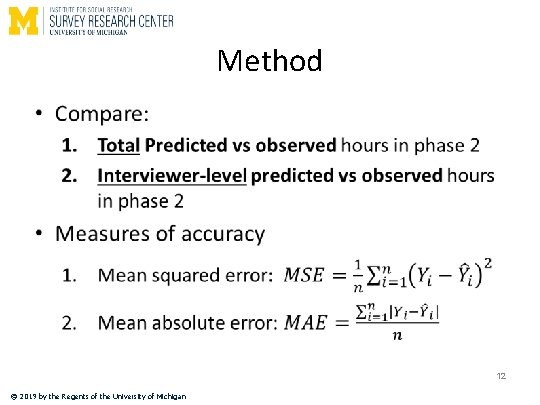
Method • 12 © 2019 by the Regents of the University of Michigan

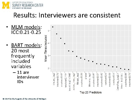
Results: Interviewers are consistent • MLM models: ICC: 0. 21‐ 0. 25 • BART models: 20 most frequently included variables – 11 are interviewer IDs 13 © 2019 by the Regents of the University of Michigan

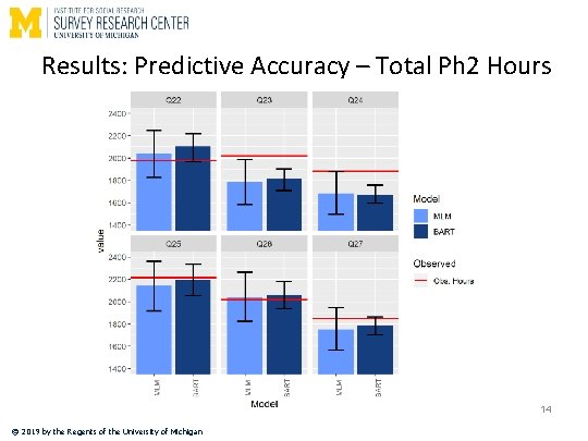
Results: Predictive Accuracy – Total Ph 2 Hours 14 © 2019 by the Regents of the University of Michigan

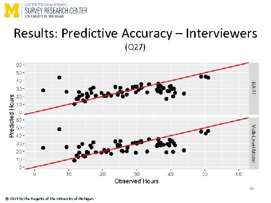
Results: Predictive Accuracy – Interviewers (Q 27) 15 © 2019 by the Regents of the University of Michigan

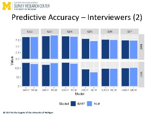
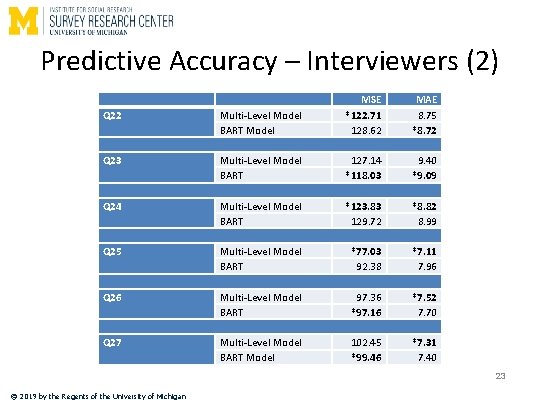
Predictive Accuracy – Interviewers (2) 16 © 2019 by the Regents of the University of Michigan

Conclusions • Cost prediction is an interesting problem • Existing methods for prediction can be used • In this problem, knowing the interviewer is very useful since their behavior is consistent • For this problem, MLM and BART models produce comparable predictive accuracy 17 © 2019 by the Regents of the University of Michigan

Thank You! • Email: jameswag@umich. edu 18 © 2019 by the Regents of the University of Michigan

References • Chipman, H. A. , E. I. George and R. E. Mc. Culloch (2010). "BART: Bayesian additive regression trees. " The Annals of Applied Statistics 4(1): 266298. • Groves, R. M. and S. G. Heeringa (2006). "Responsive design for household surveys: tools for actively controlling survey errors and costs. " Journal of the Royal Statistical Society: Series A (Statistics in Society) 169(3): 439 -457. • Wagner, J. (2019). "Estimation of Survey Cost Parameters Using Paradata. " Survey Practice 12(1): 1 -10. 19 © 2019 by the Regents of the University of Michigan

Data Source Predictor NEWIWERID TIMESHEETS NHOURS_LAG 2 TRAVEL_LAG 2 SAMPLING FRAME Description Interviewer ID Number of hours worked by the interviewer in the week two weeks prior to the current week How much did the interviewer participate in overnight travel in the week two weeks prior to the current week: NONE, SOME, or ALL week. DAYS_WORKED_LAG 2 The number of days worked (i. e. days with an entry in the timesheet) in the week two weeks prior to the current week QTR The quarter of production (Q 1‐Q 27) YEAR The calendar year of production (2011‐ 2018) CENSUS_DIV_MODE_L The modal Census Division of the lines attempted by an interviewer in the week two weeks prior to the current week AG 2 CENS_REG_MODE The modal Census Region of the lines attempted by an interviewer in the week two weeks prior to the current week _LAG 2 EST_ELIG_RATE_MEAN This is the mean of the Census Block Group level data about the estimated eligibility rate. The data are at the Block _LAG 2 Group level, but the value here is the average over all contact attempts for the week that is two weeks prior to the current week. EST_ELIG_15_49_ACS_ The mean of the estimated eligibility rate for the Census Block Group reported in the American Community Survey. The MEAN_LAG 2 data are at the Block Group level, but the value here is the average over all contact attempts for the week that is two weeks prior to the current week. ELIG_NEVER_PCT_MEA This is the percentage of eligible persons living in the Census Tract who have never been married. The data are at the N_LAG 2 Tract level, but the value here is the average over all contact attempts for the week that is two weeks prior to the current week. OCC_RATE_MEAN_LAG This is the Census Block Group level occupancy rate. The data are at the Block Group level, but the value here is the 2 average over all contact attempts for the week that is two weeks prior to the current week. DOMAIN_MODE_LAG 2 The domain is set at the Census Block Group (BG) level and assigned to housing units within each BG. All BGs are assigned to a domain based upon the following definitions: 1) <10% of Block Group African‐American and <10% Hispanic, 2) >=10% of Block Group African‐American and <10% Hispanic, 3) <10% of Block Group African‐American and >=10% Hispanic, and 4) >=10% of Block Group African‐American and >=10% Hispanic. The mode is for the domain of the lines that are attempted in the week two weeks prior to the current week URBAN_MODE_LAG 2 The mode of the urbanicity (assigned at the case level) of the attempts made during the week that is two weeks prior to the current week, where 1=Major Metropolitan Area, 2=Minor Metropolitan Area, 3=Non‐Metropolitan Area, 4=Remote 20 Area. © 2019 by the Regents of the University of Michigan

Data Source Predictor Description INTERVIEWER STRUCTURE_TYPE_MODE _LAG 2 The mode of the structure type variable of the cases that were attempted in the week that is two weeks prior to the current week. 1=Single family home, 2=Structure with 2 to 9 units, 3=Structure with 10+ units, 4= Mobile home, 5=Other. OBSERVATIONS BLACCESS_GATED_MEAN_LAG 2 The mean of an area segment‐level observation about whethere is a gated community in the area segment. This is observed at the segment level but the value here is average over all contact attempts for the week that is two weeks prior to the current week. BLACCESS_SEASONAL_HAZARD_M The mean of an area segment‐level observation about whethere is a potential seasonal hazard preventing access to the area segment (e. g. unplowed roads). This is observed at the segment level but the value here is average over all contact attempts for the week that is two weeks EAN_LAG 2 prior to the current week. BLACCESS_UNIMPROVED_ROADS_ The mean of an area segment‐level observation about whethere are unimproved roads limiting access to the area segment. This is observed at the segment level but the value here is average over all contact attempts for the week that is two weeks prior to the current week. MEAN_LAG 2 BLACCESS_OTHER_MEAN The mean of an area segment‐level observation about whethere other (i. e. not gated, seasonal hazards, or unimproved roads) factors limiting access to the area segment. This is observed at the segment level but the value here is average over all contact attempts for the week that is two weeks prior to the current week. LRESIDENTIAL_MEAN The mean of an area segment‐level observation about whether the area is completely residential or also includes some commercial structures. This is observed at the segment level but the value here is average over all contact attempts for the week that is two weeks prior to the current week. The mean of an area segment‐level observation about whether the area has evidence of non‐English speakers. This is observed at the segment level but the value here is average over all contact attempts for the week that is two weeks prior to the current week INON_ENGLISH_SPEAKERS_MEAN _LAG 2 BLNON_ENGLISH_LANG_SPANIS_ MEAN_LAG 2 The mean of an area segment‐level observation about whether the area has evidence of Spanish speakers. This is observed at the segment level but the value here is average over all contact attempts for the week that is two weeks prior to the current week. ISAFETY_CONCERNS_MEAN_LAG 2 The mean of an area segment‐level observation about whether the interviewer had concerns about their safety on the first visit. This is observed at the segment level but the value here is average over all contact attempts for the week that is two weeks prior to the current week. MANYUNITS_MEAN_LAG 2 The mean of an observation at the housing unit level indicating whether the sampled housing unit has 1=more than one unit, or 0=1 unit. This is observed at the housing unit level but the value here is average over all contact attempts for the week that is two weeks prior to the current week. The mean of an observation at the housing unit level indicating whether the interviewer believes that there are children under the age of 15 living in the housing unit (1=Yes, 0=No). This is observed at the housing unit level but the value here is average over all contact attempts for the week that is two weeks prior to the current week. CHILDRENUNDER 15_MEAN_LAG 2 ALLAGEOVER 45_MEAN_LAG 2 The mean of an observation at the housing unit level indicating whether the interviewer believes that persons living in the housing unit are all over the age of 45 (1=Yes, 0=No). This is observed at the housing unit level but the value here is average over all contact attempts for the week that is two weeks prior to the current week. 21 © 2019 by the Regents of the University of Michigan

Data Source Predictor Description COMMERCIAL MSG_MATCHQUALITY_MEAN_ A variable indicating the estimated quality of the match of commercially‐available data to the address (1‐ 5). The data are at the case level, but the value here is the average over all contact attempts for the week that is two weeks prior to the current week. DATA LAG 2 The mean age of the first person from the commercially‐available data where those data are available. The data are at the case level, but the MSG_AGE_MEAN_LAG 2 MSG_INCOME_MEAN_LAG 2 LEVEL OF EFFORT PARADATA PHASE LAG 2. ACTIVE_LINES TRIPS_LAG 2 FTFNOCONTACT_LAG 2 FTFAPPT_LAG 2 MAINIW_LAG 2 FTFMAINRESIST_LAG 2 FTFMAINNI_LAG 2 FTFMAINNS_LAG 2 FTFSCRNIW_LAG 2 FTFSCRNRESIST_LAG 2 FTFSCRNNI_LAG 2 FTFSCRNNS_LAG 2 FTF_MAINNS_INEL_LAG 2 ACTIVE_LINES_LAG 2 TEL_ALL_LAG 2 value here is the average over all contact attempts for the week that is two weeks prior to the current week The mean of the estimated household income for cases with a match to commercially‐available data. The data are at the case level, but the value here is the average over all contact attempts for the week that is two weeks prior to the current week The phase of the NSFG design (first phase occurs in weeks 1‐ 10, phase 2 during weeks 11‐ 12). The number of active lines from 2 weeks prior to the current week for each interviewer. The total number of unique visits to an area segment (derived from call record data) from 2 weeks prior to the current week for each interviewer. The total number of Face‐to‐face contact attempts that resulted in no contact from 2 weeks prior to the current week for each interviewer. The total number of Face‐to‐face contact attempts that resulted in a contact with only agreement for a general callback from 2 weeks prior to the current week for each interviewer. The total number of Face‐to‐face contact attempts that resulted in setting an appointment from 2 weeks prior to the current week for each interviewer. The total number of main interviews (all main interviews are completed face‐to‐face) from 2 weeks prior to the current week for each interviewer. The total number of Face‐to‐face contact attempts that resulted in the sampled person expressing concerns from 2 weeks prior to the current week for each interviewer. The total number of Face‐to‐face contact attempts that resulted in a final noninterview from 2 weeks prior to the current week for each interviewer. The total number of Face‐to‐face contact attempts that resulted in a final nonsample from 2 weeks prior to the current week for each interviewer. The total number of Face‐to‐face contact attempts that resulted in a screening interview from 2 weeks prior to the current week for each interviewer. The total number of Face‐to‐face contact attempts that resulted in the sampled housing unit expressing concerns prior to completing a screening interview from 2 weeks prior to the current week for each interviewer. The total number of Face‐to‐face contact attempts that resulted in the sampled housing unit being finalized as a noninterview prior to completing a screening interview from 2 weeks prior to the current week for each interviewer. The total number of Face‐to‐face contact attempts that resulted in the sampled housing unit being finalized as nonsample prior to completing a screening interview from 2 weeks prior to the current week for each interviewer. The total number of Face‐to‐face contact attempts that resulted in the sampled person being finalized as ineligible prior to completing a screening interview from 2 weeks prior to the current week for each interviewer. The number of active sampled units two weeks prior to the current week for each interviewer. The total number of telephone attempts made by each interviewer two weeks prior to the current week. © 2019 by the Regents of the University of Michigan 22

Predictive Accuracy – Interviewers (2) Q 22 Multi‐Level Model BART Model MSE *122. 71 128. 62 MAE 8. 75 *8. 72 Q 23 Multi‐Level Model BART 127. 14 *118. 03 9. 40 *9. 09 Q 24 Multi‐Level Model BART *123. 83 129. 72 *8. 82 8. 99 Q 25 Multi‐Level Model BART *77. 03 92. 38 *7. 11 7. 96 Q 26 Multi‐Level Model BART 97. 36 *97. 16 *7. 52 7. 70 Q 27 Multi‐Level Model BART Model 102. 45 *99. 46 *7. 31 7. 40 23 © 2019 by the Regents of the University of Michigan