Using Local Moment Invariants for Partial 3 D

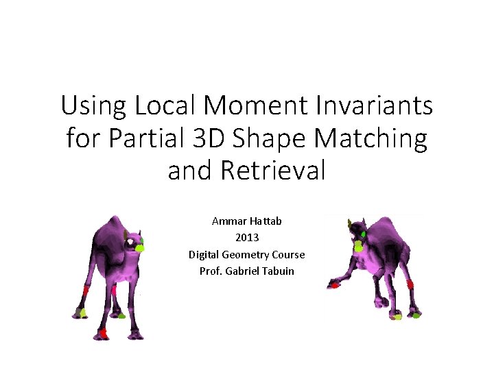
Using Local Moment Invariants for Partial 3 D Shape Matching and Retrieval Ammar Hattab 2013 Digital Geometry Course Prof. Gabriel Tabuin

Project Goal • Moment Invariants are normally used as Global shape descriptors. • The goal of this project is to use them as a Local shape descriptor. • And to build a 3 D shape retrieval and matching system based on moment invariants.

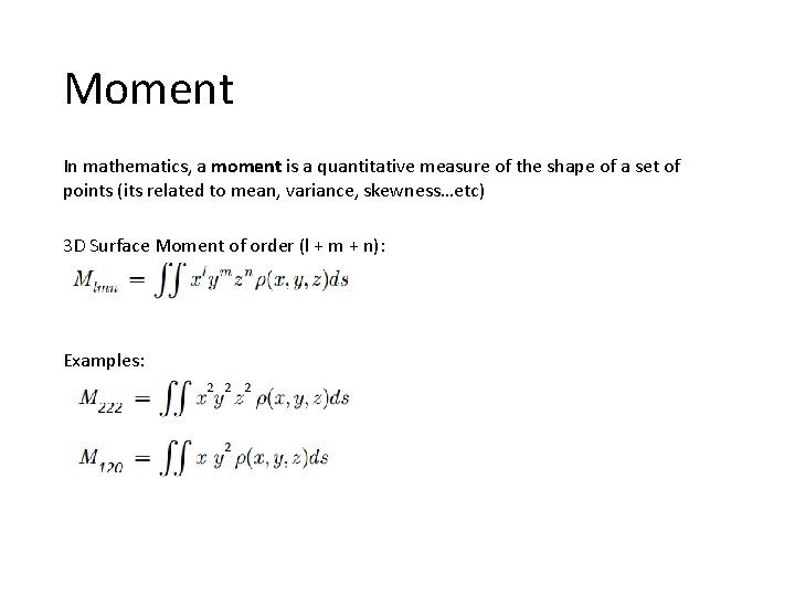
Moment In mathematics, a moment is a quantitative measure of the shape of a set of points (its related to mean, variance, skewness…etc) 3 D Surface Moment of order (l + m + n): Examples:

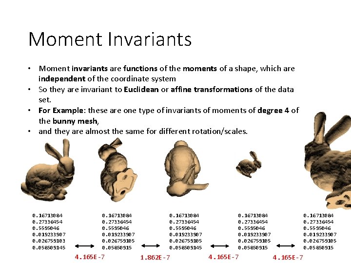
Moment Invariants • Moment invariants are functions of the moments of a shape, which are independent of the coordinate system • So they are invariant to Euclidean or affine transformations of the data set. • For Example: these are one type of invariants of moments of degree 4 of the bunny mesh, • and they are almost the same for different rotation/scales. 0. 16713084 0. 27336454 0. 5595046 0. 019233907 0. 026759103 0. 058509145 0. 16713084 0. 27336454 0. 5595046 0. 019233907 0. 026759105 0. 05850915 4. 165 E-7 0. 16713084 0. 27336454 0. 5595046 0. 019233907 0. 026759105 0. 058509145 1. 862 E-7 0. 16713084 0. 27336454 0. 5595046 0. 019233907 0. 026759105 0. 05850915 4. 165 E-7

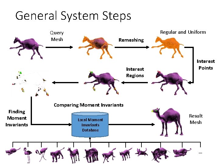
General System Steps Regular and Uniform Query Mesh Remeshing Interest Regions Finding Moment Invariants Interest Points Comparing Moment Invariants Local Moment Invariants Database Result Mesh …

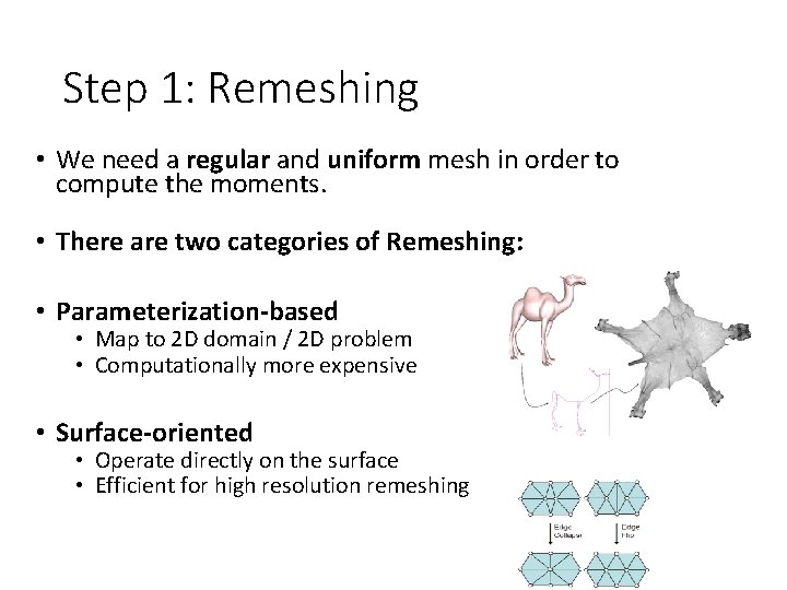
Step 1: Remeshing • We need a regular and uniform mesh in order to compute the moments. • There are two categories of Remeshing: • Parameterization-based • Map to 2 D domain / 2 D problem • Computationally more expensive • Surface-oriented • Operate directly on the surface • Efficient for high resolution remeshing

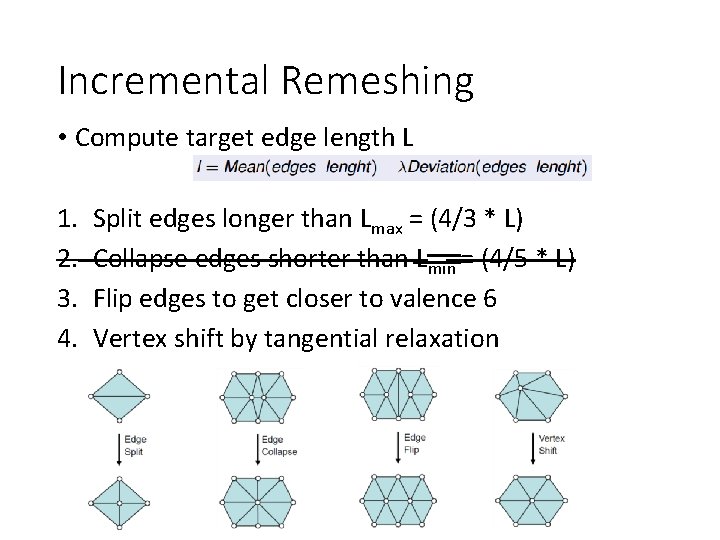
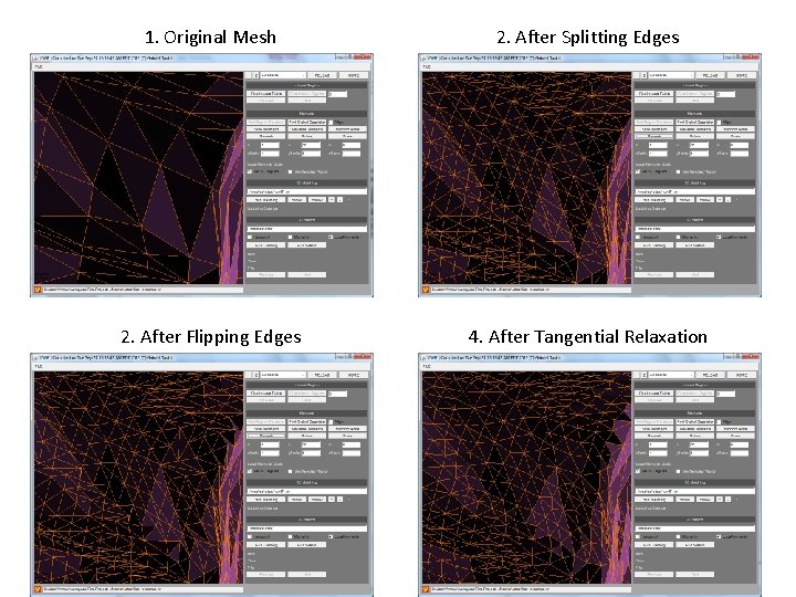
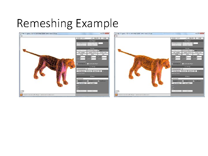
Incremental Remeshing • Compute target edge length L 1. 2. 3. 4. Split edges longer than Lmax = (4/3 * L) Collapse edges shorter than Lmin = (4/5 * L) Flip edges to get closer to valence 6 Vertex shift by tangential relaxation

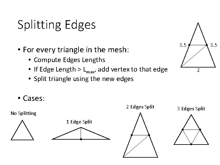
Splitting Edges • For every triangle in the mesh: • Compute Edges Lengths • If Edge Length > Lmax, add vertex to that edge • Split triangle using the new edges 3. 5 2 • Cases: 2 Edges Split No Splitting 1 Edge Split 3 Edges Split

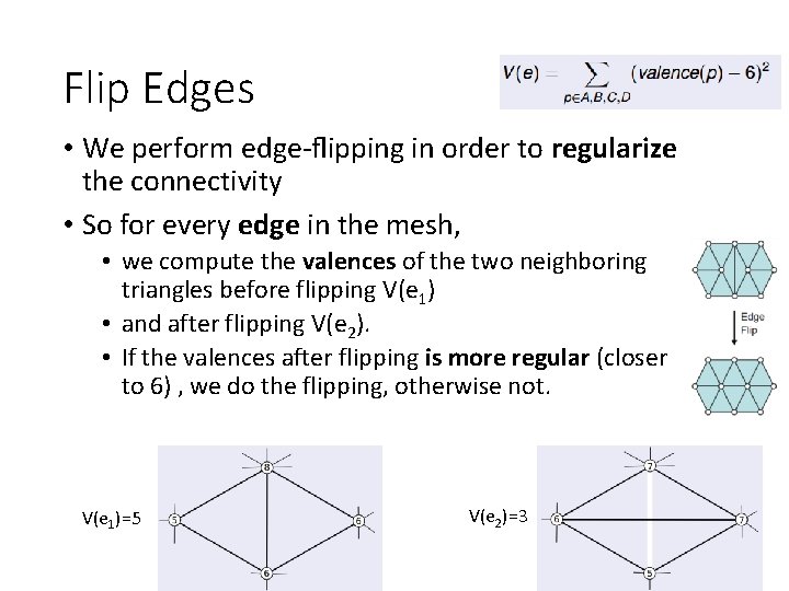
Flip Edges • We perform edge‐flipping in order to regularize the connectivity • So for every edge in the mesh, • we compute the valences of the two neighboring triangles before flipping V(e 1) • and after flipping V(e 2). • If the valences after flipping is more regular (closer to 6) , we do the flipping, otherwise not. V(e 1)=5 V(e 2)=3

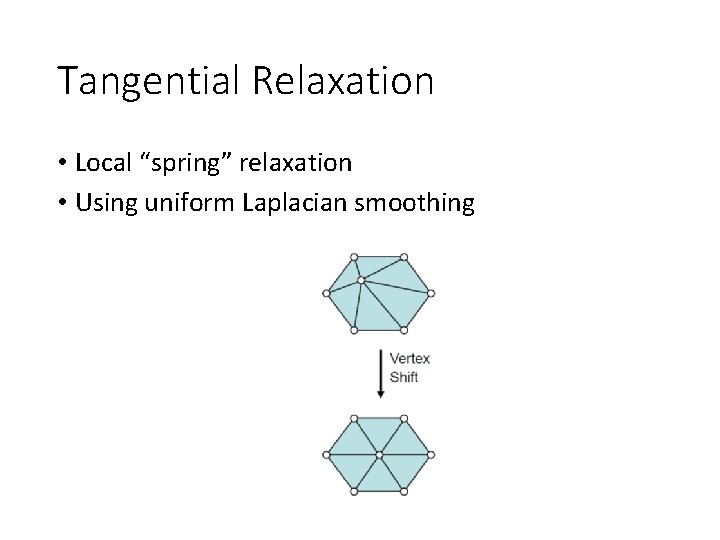
Tangential Relaxation • Local “spring” relaxation • Using uniform Laplacian smoothing

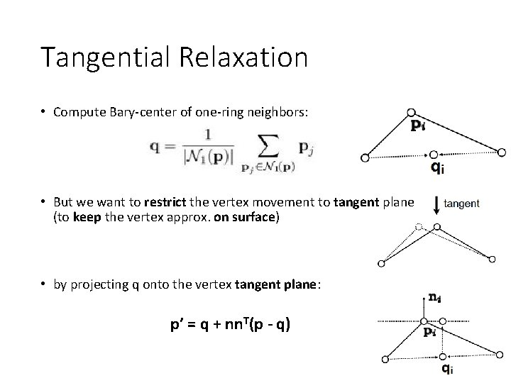
Tangential Relaxation • Compute Bary‐center of one‐ring neighbors: • But we want to restrict the vertex movement to tangent plane (to keep the vertex approx. on surface) • by projecting q onto the vertex tangent plane: p’ = q + nn. T(p - q)

1. Original Mesh 2. After Splitting Edges 2. After Flipping Edges 4. After Tangential Relaxation

Remeshing Example

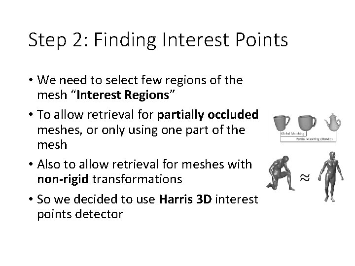
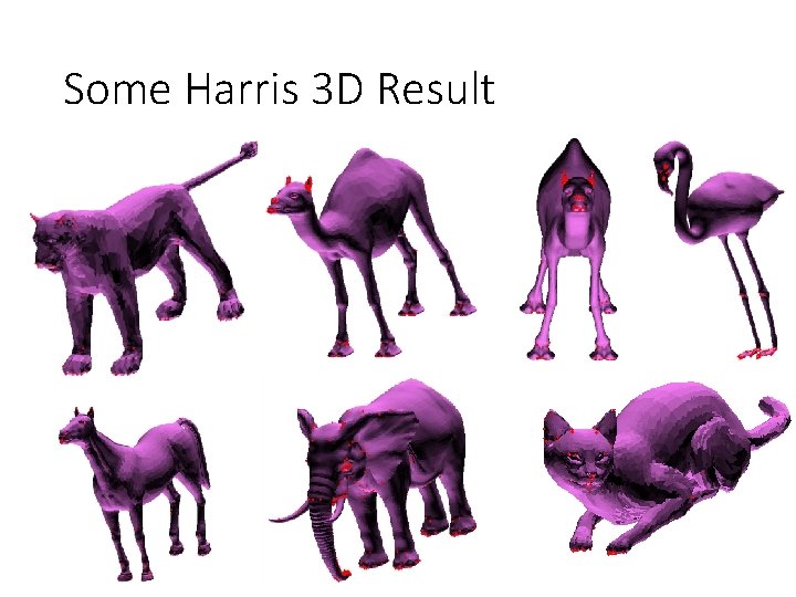
Step 2: Finding Interest Points • We need to select few regions of the mesh “Interest Regions” • To allow retrieval for partially occluded meshes, or only using one part of the mesh • Also to allow retrieval for meshes with non-rigid transformations • So we decided to use Harris 3 D interest points detector

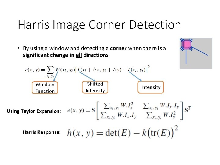
Harris Image Corner Detection • By using a window and detecting a corner when there is a significant change in all directions Window Function Using Taylor Expansion: Harris Response: Shifted Intensity

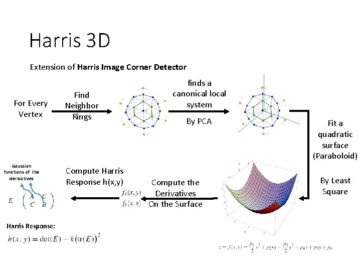
Harris 3 D Extension of Harris Image Corner Detector For Every Vertex Gaussian functions of the derivatives Harris Response: Find Neighbor Rings Compute Harris Response h(x, y) finds a canonical local system By PCA Compute the Derivatives On the Surface Fit a quadratic surface (Paraboloid) By Least Square

Some Harris 3 D Result

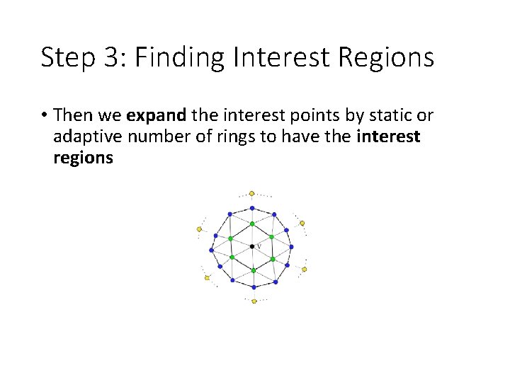
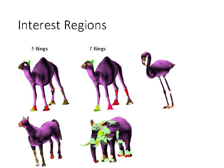
Step 3: Finding Interest Regions • Then we expand the interest points by static or adaptive number of rings to have the interest regions

Interest Regions 5 Rings 7 Rings

Step 4: Moment Invariants • We need to have an efficient method with low computational cost. • As shown in [Taubin 1991], We could store moments in Matrices, and apply efficient matrix operations such as (computation of Eigen Values) to get the Moment Invariants.

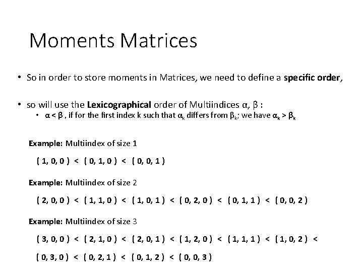
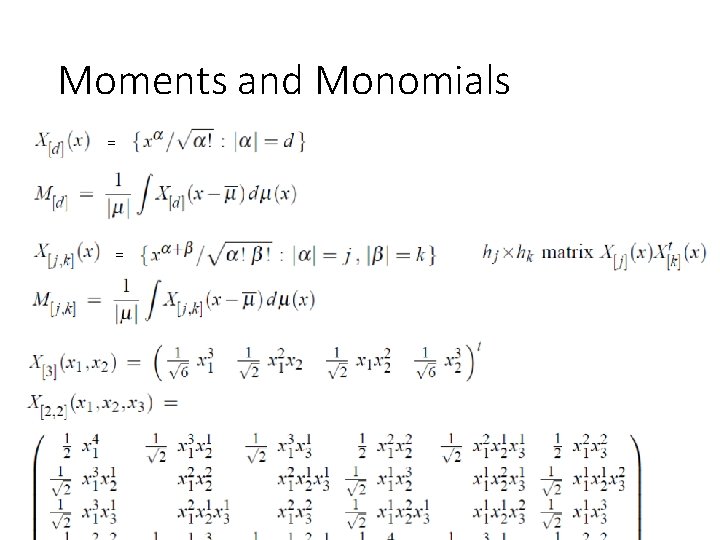
Moments Matrices • So in order to store moments in Matrices, we need to define a specific order, • so will use the Lexicographical order of Multiindices α, β : • α < β , if for the first index k such that αk differs from βk; we have αk > βk Example: Multiindex of size 1 ( 1, 0, 0 ) < ( 0, 1, 0 ) < ( 0, 0, 1 ) Example: Multiindex of size 2 ( 2, 0, 0 ) < ( 1, 1, 0 ) < ( 1, 0, 1 ) < ( 0, 2, 0 ) < ( 0, 1, 1 ) < ( 0, 0, 2 ) Example: Multiindex of size 3 ( 3, 0, 0 ) < ( 2, 1, 0 ) < ( 2, 0, 1 ) < ( 1, 2, 0 ) < ( 1, 1, 1 ) < ( 1, 0, 2 ) < ( 0, 3, 0 ) < ( 0, 2, 1 ) < ( 0, 1, 2 ) < ( 0, 0, 3 )

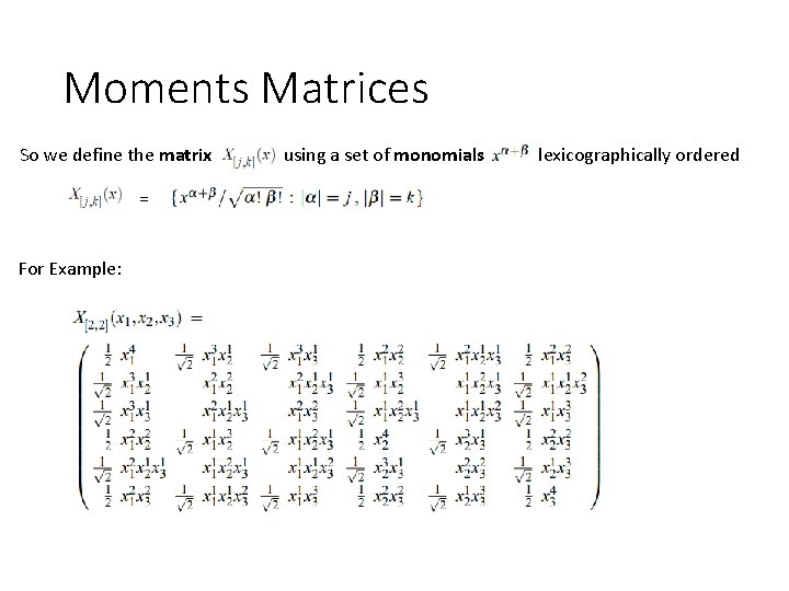
Moments Matrices So we define the matrix using a set of monomials lexicographically ordered = For Example:

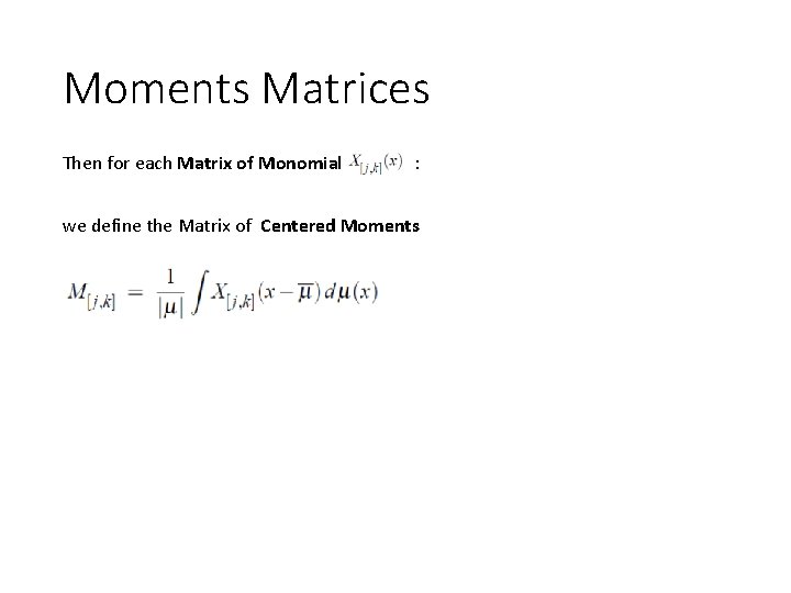
Moments Matrices Then for each Matrix of Monomial : we define the Matrix of Centered Moments

Example: Computing M[2, 2] • Initialize moments matrix M[2, 2] ( 6 × 6 ) to zeros. • For Every Triangle in the Mesh • • Get Triangle vertices coordinates x 1, y 1, z 1, x 2, y 2, z 2, x 3, y 3, z 3. Compute Triangle Area Compute Matrix of Monomials as described before Add Matrix to M[2, 2] • Normalize, matrix M[2, 2] by dividing on total triangles area. • Compute Eigen values of M[2, 2] by using Eigen value decomposition (provided by Jama package) • These are the Moment Invariants

Example: Computing M[2, 2] • So In the example of the bunny mesh, these are the Eigen Values of Eigen Values 0. 16713084 0. 27336454 0. 5595046 0. 019233907 0. 026759103 0. 058509145 and Eigen Values 0. 16713084 0. 27336454 0. 5595046 0. 019233907 0. 026759105 0. 05850915 0. 16713084 0. 27336454 0. 5595046 0. 019233907 0. 026759105 0. 058509145 0. 16713084 0. 27336454 0. 5595046 0. 019233907 0. 026759105 0. 05850915 4. 165 E-7 1. 862 E-7 4. 165 E-7

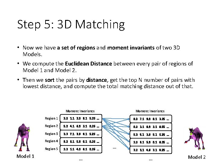
Step 5: 3 D Matching • Now we have a set of regions and moment invariants of two 3 D Models. • We compute the Euclidean Distance between every pair of regions of Model 1 and Model 2. • Then we sort the pairs by distance, get the top N number of pairs with lowest distance, and compute the total matching distance out of that. Model 1 Moment Invariants Region 1 3. 2 1. 1 3. 9 8. 1 5. 25 … 8. 2 7. 1 9. 9 8. 1 3. 25 … Region 2 5. 2 4. 1 6. 9 3. 1 0. 25 … 0. 2 3. 1 6. 9 3. 1 0. 55 … Region 3 3. 3 7. 1 3. 9 8. 1 5. 25 … 5. 3 5. 1 3. 9 5. 1 5. 25 … Region 4 9. 2 8. 1 5. 9 0. 1 0. 25 … 2. 2 8. 1 5. 9 0. 1 0. 25 … Region 5 2. 2 1. 1 4. 9 8. 1 0. 25 … … … 3. 2 1. 1 4. 9 3. 1 0. 25 … … Model 2

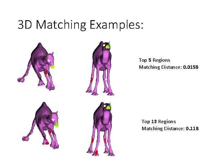
3 D Matching Examples: Top 5 Regions Matching Distance: 0. 0158 Top 13 Regions Matching Distance: 0. 118

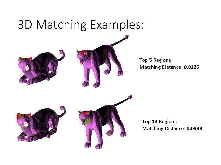
3 D Matching Examples: Top 5 Regions Matching Distance: 0. 0225 Top 13 Regions Matching Distance: 0. 0939

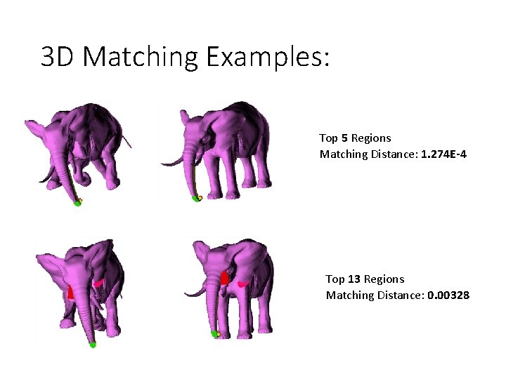
3 D Matching Examples: Top 5 Regions Matching Distance: 1. 274 E-4 Top 13 Regions Matching Distance: 0. 00328

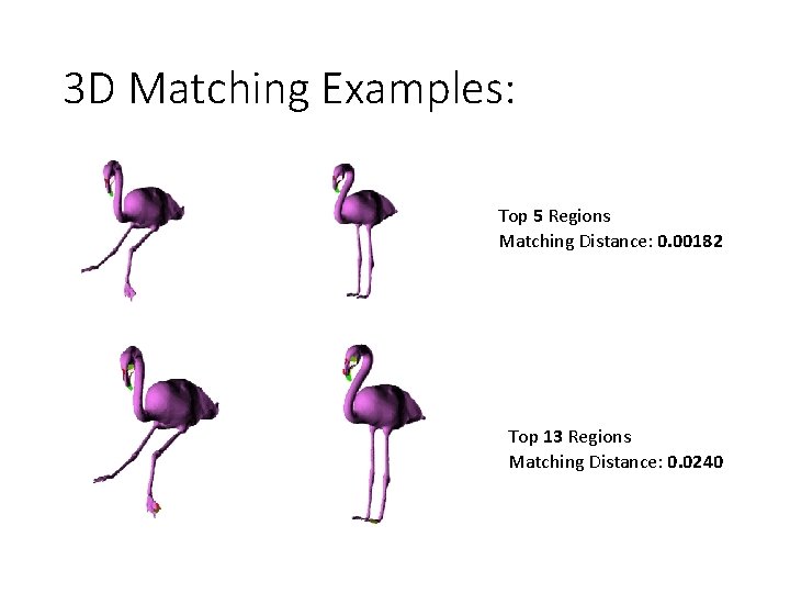
3 D Matching Examples: Top 5 Regions Matching Distance: 0. 00182 Top 13 Regions Matching Distance: 0. 0240

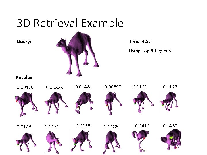
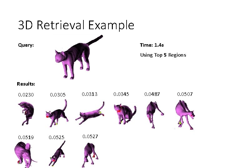
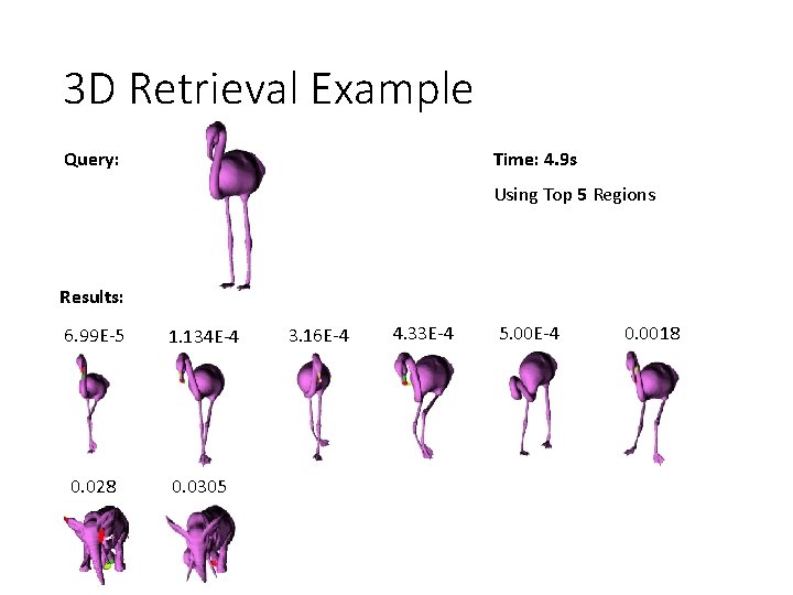
Step 6: 3 D Retrieval • The 3 D retrieval is performed by computing the matching distance between a query 3 D model and every other 3 D model in the database • Then sort the search results by matching distance

3 D Retrieval Example Query: Time: 4. 8 s Using Top 5 Regions Results: 0. 00129 0. 00323 0. 00481 0. 00597 0. 0128 0. 0151 0. 0158 0. 0185 0. 0120 0. 0419 0. 0127 0. 0452

3 D Retrieval Example Query: Time: 1. 4 s Using Top 5 Regions Results: 0. 0230 0. 0305 0. 0313 0. 0519 0. 0525 0. 0527 0. 0345 0. 0487 0. 0507

3 D Retrieval Example Query: Time: 4. 9 s Using Top 5 Regions Results: 6. 99 E‐ 5 1. 134 E‐ 4 0. 028 0. 0305 3. 16 E‐ 4 4. 33 E‐ 4 5. 00 E‐ 4 0. 0018

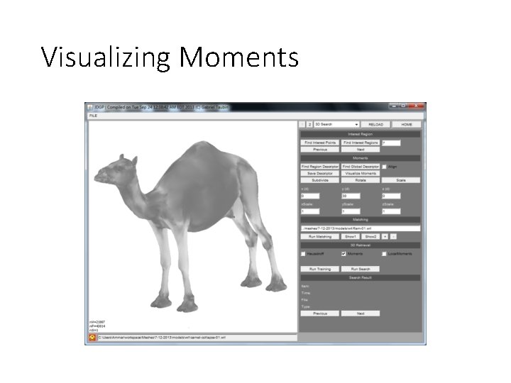
Visualizing Moments

Conclusions • Using Matrix operations for calculating moment invariants is a very fast and efficient algorithm. • On my tests, the query time was 1 -6 seconds depending on the complexity of the model and the size of the database. • This is very fast compared to brute force search; using Haussdroff distance for example which takes several minutes for a database of 100 models. • A large portion of the query time was taken by the interest points detector. • So although Harris 3 D is an accurate interest points detector, its performance could be enhanced.

Future Steps • Trying to use Moment Invariants for interest points and regions detection • Using space partitioning algorithms (ex: like ANN) to efficiently find the nearest features of a database of features. • Compare the performance of moment invariants as a local descriptor with other local descriptors

Main References • Data Set: • Sumner, Robert W. , and Jovan Popović. Mesh Data from Deformation Transfer for Triangle Meshes. (2004) • http: //people. csail. mit. edu/sumner/research/deftransfer/data. html • Taubin, Gabriel, and David B. Cooper. Object recognition based on moment (or algebraic) invariants. IBM TJ Watson Research Center, 1991. • Zhang, Cha, and Tsuhan Chen. "Efficient feature extraction for 2 D/3 D objects in mesh representation. " Image Processing, 2001. Proceedings. 2001 International Conference on. Vol. 3. IEEE, 2001. • Sipiran, Ivan, and Benjamin Bustos. "Harris 3 D: a robust extension of the Harris operator for interest point detection on 3 D meshes. " The Visual Computer 27. 11 (2011): 963‐ 976. • Botsch, Mario, et al. Polygon mesh processing. P. 100: Incremental Remeshing. 2010. • Liu, Zhen‐Bao, et al. "A Survey on Partial Retrieval of 3 D Shapes. " Journal of Computer Science and Technology 28. 5 (2013): 836‐ 851. • Lindsay I Smith. “A tutorial on Principal Components Analysis”. 2002

Extra References • Alliez, Pierre, et al. "Isotropic surface remeshing. " Shape Modeling International, 2003. IEEE, 2003. • Prokop, Richard J. , and Anthony P. Reeves. "A survey of moment‐based techniques for unoccluded object representation and recognition. " CVGIP: Graphical Models and Image Processing 54. 5 (1992): 438‐ 460. • Tangelder, Johan WH, and Remco C. Veltkamp. "A survey of content based 3 D shape retrieval methods. " Multimedia tools and applications 39. 3 (2008): 441‐ 471. • Kazhdan, Michael M. Shape representations and algorithms for 3 D model retrieval. Diss. Princeton University, 2004. • Sipiran, Ivan, and Benjamin Bustos. "Key‐components: detection of salient regions on 3 D meshes. " The Visual Computer 29. 12 (2013): 1319‐ 1332. • Sun, Jian, Maks Ovsjanikov, and Leonidas Guibas. "A Concise and Provably Informative Multi‐Scale Signature Based on Heat Diffusion. " Computer Graphics Forum. Vol. 28. No. 5. Blackwell Publishing Ltd, 2009. • http: //www. astro. utu. fi/edu/kurssit/f 90/english/pdf/numfit 2. pdf

END

Backup Slides

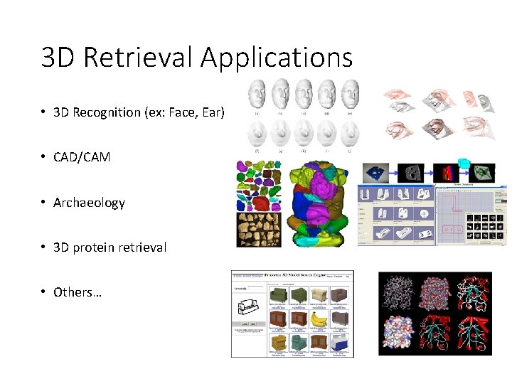
3 D Retrieval Applications • 3 D Recognition (ex: Face, Ear) • CAD/CAM • Archaeology • 3 D protein retrieval • Others…

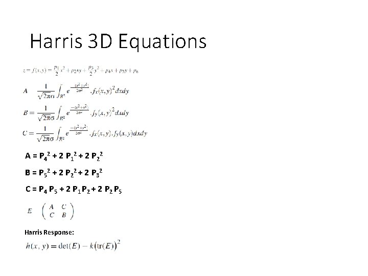
Harris 3 D • Our algorithm works in a vertex‐wise manner in order to compute the Harris response for each vertex: • It determines a neighborhood for each vertex. It can be spatial, adaptive or ring neighborhoods. • It finds a canonical local system by applying PCA to the neighborhood. • It fits a quadratic surface on the normalized neighborhood. • It computes derivatives on the fitted surface. Gaussian functions are used for smoothing the derivatives. By using integration between the derivatives and the gaussians, the method is robust to local geometric changes. • Using the derivatives, the algorithm constructs the auto‐ correlation function needed to evaluate the Harris operator. Subsequently, a response is computed for each vertex.

Descriptors • Measuring similarity • In order to measure how similar two objects are, it is necessary to compute distances between pairs of descriptors using a dissimilarity measure • Efficiency • For large shape collections, it is inefficient to sequentially match all objects in the database with the query object. Because retrieval should be fast, efficient indexing search structures are needed to support efficient retrieval

Descriptors • Discriminative power: • A shape descriptor should capture properties that discriminate objects well • Robustness and sensitivity • It is often desirable that a shape descriptor is insensitive to noise and small extra features, and robust against arbitrary topological degeneracies, e. g. if it is obtained by laser scanning

How we used moment invariants • The matching of arbitrarily shaped regions is done by computing for each region a vector of centered moments. These vectors are viewpoint dependent, but the dependence on the viewpoint is algebraic and well known. We then compute moment invariants, i. e. , algebraic functions of the moments that are invariant to Euclidean or affine transformations of the data set

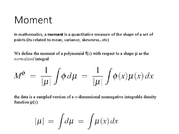
Moment In mathematics, a moment is a quantitative measure of the shape of a set of points (its related to mean, variance, skewness…etc) We define the moment of a polynomial f(x) with respect to a shape μ as the normalized integral the data is a sampled version of a n-dimensional nonnegative integrable density function μ(x)

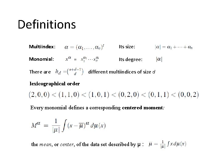
Definitions Multiindex: Monomial: Its size: = There are Its degree: different multiindices of size d lexicographical order Every monomial defines a corresponding centered moment: the mean, or center, of the data set described by μ :

Moments and Monomials = =

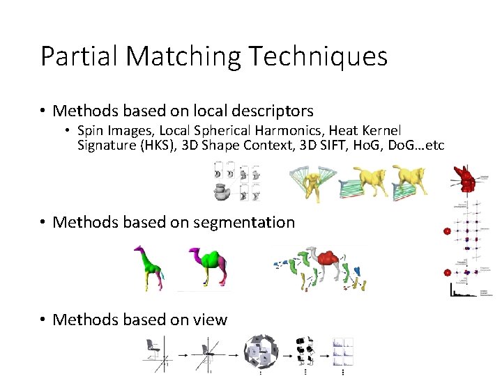
Partial Matching Techniques • Methods based on local descriptors • Spin Images, Local Spherical Harmonics, Heat Kernel Signature (HKS), 3 D Shape Context, 3 D SIFT, Ho. G, Do. G…etc • Methods based on segmentation • Methods based on view

Harris 3 D Equations A = P 42 + 2 P 12 + 2 P 22 B = P 52 + 2 P 22 + 2 P 32 C = P 4 P 5 + 2 P 1 P 2 + 2 P 5 Harris Response: