Using Graph Theory to Study Neural Networks Watrous

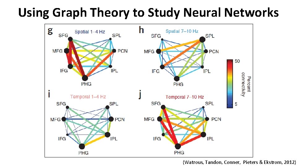
Using Graph Theory to Study Neural Networks (Watrous, Tandon, Conner, Pieters & Ekstrom, 2012)

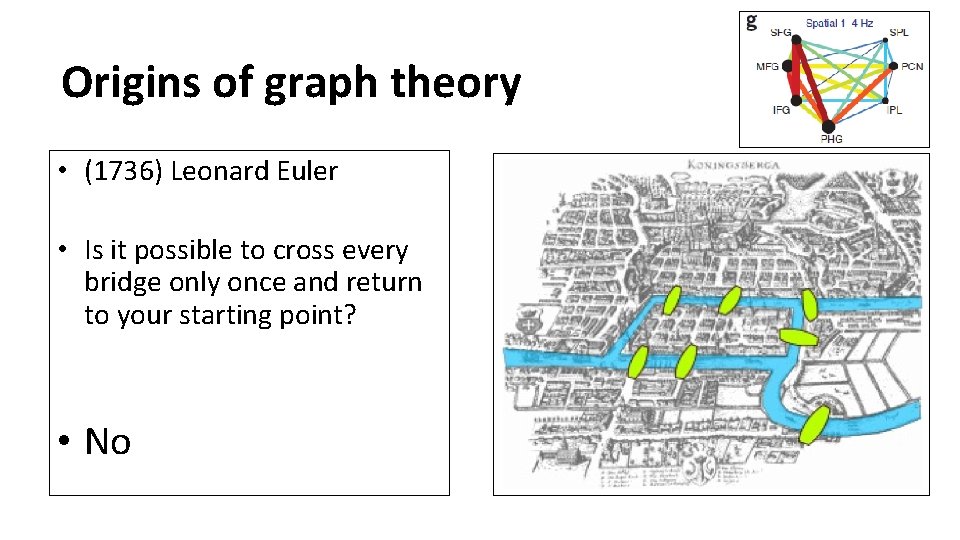
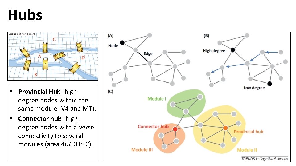
Origins of graph theory • (1736) Leonard Euler • Is it possible to cross every bridge only once and return to your starting point? • No

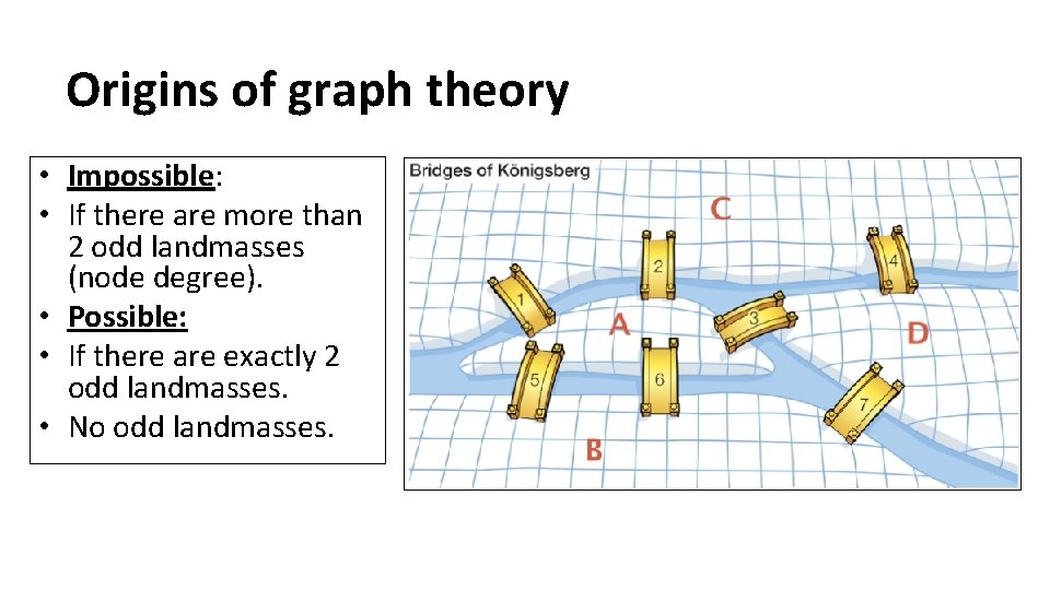
Origins of graph theory • Impossible: • If there are more than 2 odd landmasses (node degree). • Possible: • If there are exactly 2 odd landmasses. • No odd landmasses.

Definitions • Node degree: # of edges connected to a node (high degree = hub). • Cluster: when the nearest neighbors of a node are directly connected to each other (complex networks have high clustering). • Path length: minimum # of edges to get from one node to another (complex networks have short average paths). • Modules: contain many densely interconnected nodes. There are few connections between nodes in different modules.

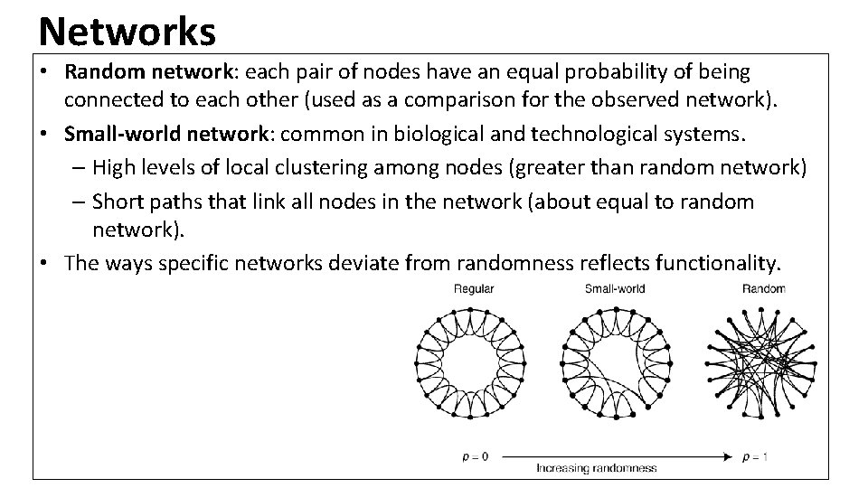
Networks • Random network: each pair of nodes have an equal probability of being connected to each other (used as a comparison for the observed network). • Small-world network: common in biological and technological systems. – High levels of local clustering among nodes (greater than random network) – Short paths that link all nodes in the network (about equal to random network). • The ways specific networks deviate from randomness reflects functionality.

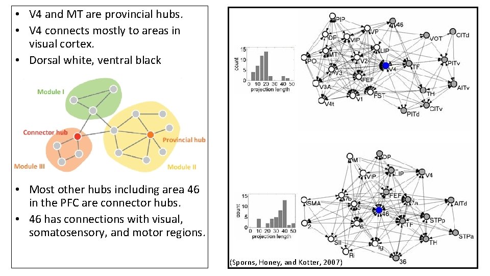
Hubs • Provincial Hub: highdegree nodes within the same module (V 4 and MT). • Connector hub: highdegree nodes with diverse connectivity to several modules (area 46/DLPFC).

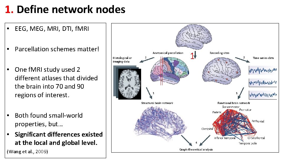
1. Define network nodes • EEG, MRI, DTI, f. MRI • Parcellation schemes matter! • One f. MRI study used 2 different atlases that divided the brain into 70 and 90 regions of interest. • Both found small-world properties, but… • Significant differences existed at the local and global level. (Wang et al. , 2009) 1

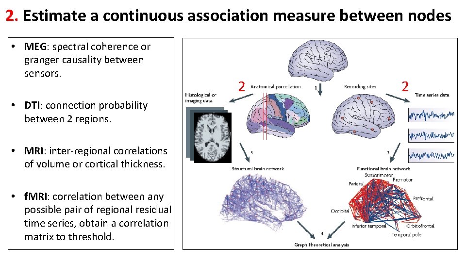
2. Estimate a continuous association measure between nodes • MEG: spectral coherence or granger causality between sensors. • DTI: connection probability between 2 regions. • MRI: inter-regional correlations of volume or cortical thickness. • f. MRI: correlation between any possible pair of regional residual time series, obtain a correlation matrix to threshold. 2 2

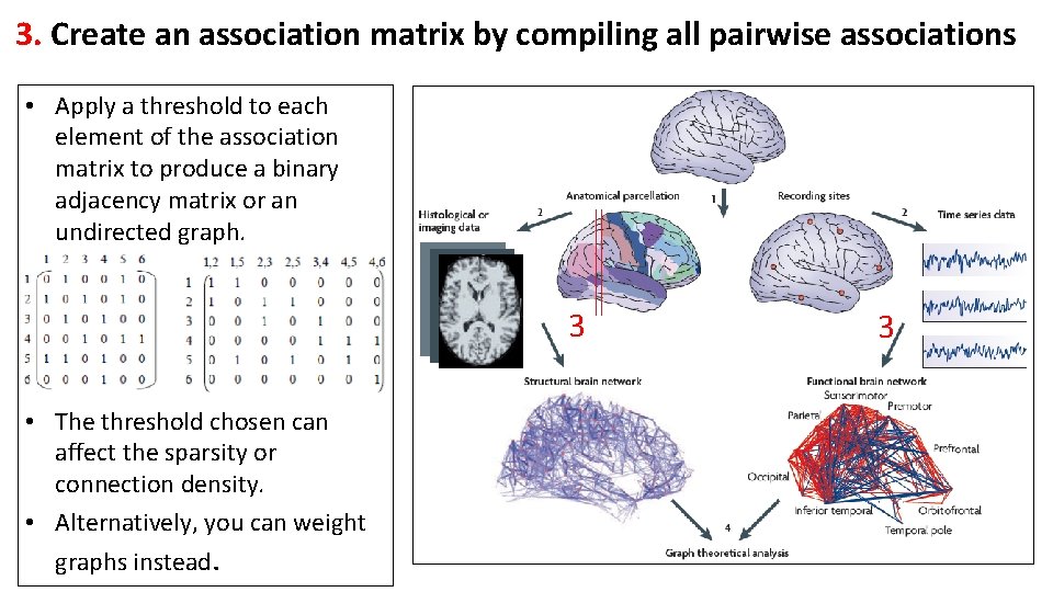
3. Create an association matrix by compiling all pairwise associations • Apply a threshold to each element of the association matrix to produce a binary adjacency matrix or an undirected graph. 3 • The threshold chosen can affect the sparsity or connection density. • Alternatively, you can weight graphs instead. 3

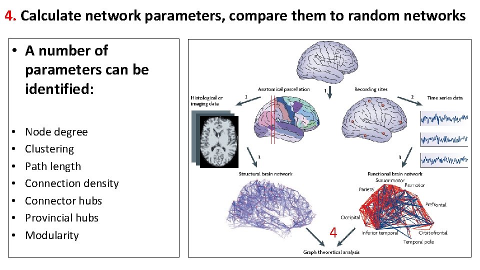
4. Calculate network parameters, compare them to random networks • A number of parameters can be identified: • • Node degree Clustering Path length Connection density Connector hubs Provincial hubs Modularity 4

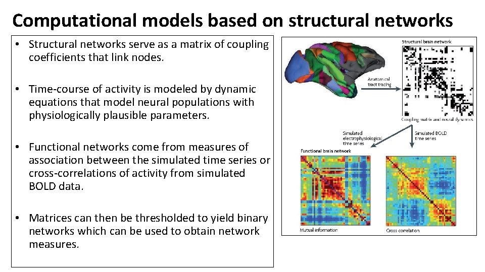
Computational models based on structural networks • Structural networks serve as a matrix of coupling coefficients that link nodes. • Time-course of activity is modeled by dynamic equations that model neural populations with physiologically plausible parameters. • Functional networks come from measures of association between the simulated time series or cross-correlations of activity from simulated BOLD data. • Matrices can then be thresholded to yield binary networks which can be used to obtain network measures.

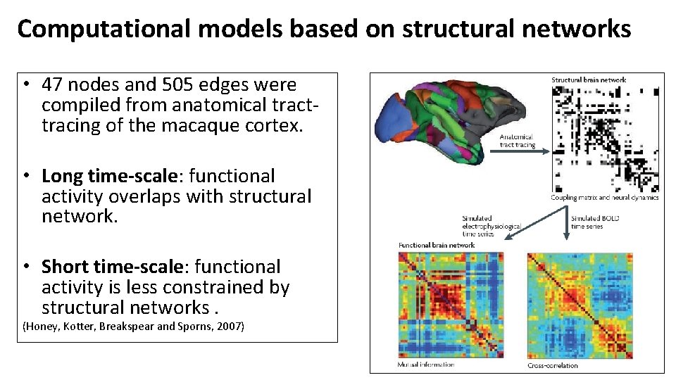
Computational models based on structural networks • 47 nodes and 505 edges were compiled from anatomical tracttracing of the macaque cortex. • Long time-scale: functional activity overlaps with structural network. • Short time-scale: functional activity is less constrained by structural networks. (Honey, Kotter, Breakspear and Sporns, 2007)

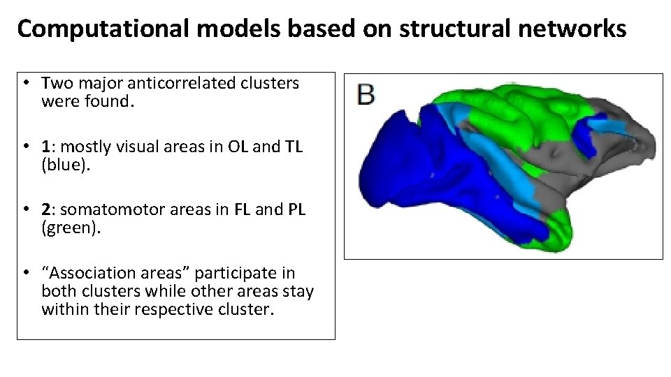
Computational models based on structural networks • Two major anticorrelated clusters were found. • 1: mostly visual areas in OL and TL (blue). • 2: somatomotor areas in FL and PL (green). • “Association areas” participate in both clusters while other areas stay within their respective cluster.

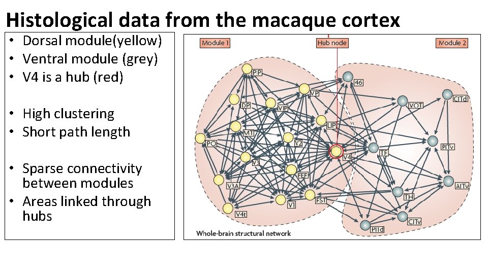
Histological data from the macaque cortex • Dorsal module(yellow) • Ventral module (grey) • V 4 is a hub (red) • High clustering • Short path length • Sparse connectivity between modules • Areas linked through hubs

• V 4 and MT are provincial hubs. • V 4 connects mostly to areas in visual cortex. • Dorsal white, ventral black • Most other hubs including area 46 in the PFC are connector hubs. • 46 has connections with visual, somatosensory, and motor regions. (Sporns, Honey, and Kotter, 2007)

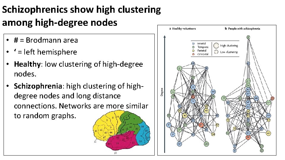
Schizophrenics show high clustering among high-degree nodes • # = Brodmann area • ‘ = left hemisphere • Healthy: low clustering of high-degree nodes. • Schizophrenia: high clustering of highdegree nodes and long distance connections. Networks are more similar to random graphs.