Using Geo DA Software for Geographic Data Analysis

Using Geo. DA Software for Geographic Data Analysis and Exploration Developed by Luc Anselin Arizona State University School of Geography and Planning geodatacenter. asu. edu 1 Briggs Henan University 2010

Software for Spatial Analysis and Statistics • Arc. GIS 9 The most common GIS Software, but $$$$! – Spatial Statistics Tools for point and polygon analysis – Spatial Analyst tools for density kernel – Geo. Statistical Analyst Tools for interpolation of continuous surface data • Open. Geo. DA, Geographic Data Analysis by Luc Anselin now at Arizona State – – Download from: http: //geodacenter. asu. edu/ Runs on Vista and Windows 7 (also MAC and UNIX) Earlier version called Geo. DA runs only on XP (0. 9. 5 i_6) Easy to use and has good graphic capabilities • Crime. Stat III download from http: //www. icpsr. umich. edu/NACJD/crimestat. html – Standalone package, free for government and education use – Calculates values for spatial statistics but no GIS graphics – Good documentation and explanation of measures and concepts • R Open Source statistical package, – – originally on UNIX but now has MS Windows version Has the most extensive set of spatial statistical analyses Difficult to use Need to learn it if you are going to do major work in this area • S-Plus the only commercial statistical package with good support for spatial 2 statistics – www. insightful. com Briggs Henan University 2010

Geo. DA Overview • Geo. DA is a package for exploratory analysis of geographic data. • Primarily analyzes polygon data, but can also do some things with point data • Has major capabilities not easily available elsewhere including: • --creates spatial weights matrices with multiple options • --linking and brushing between maps, histograms, scatter plots • --calculates and maps Local Indices of Spatial Association (LISA or local Moran’s I). • standard multiple regression full diagnostics for spatial effects • spatial autoregressive model for both spatial lag and spatial error models • Free. Arc. GIS not required, but it does require a shapefile for data input. 3 Briggs Henan University 2010

Obtaining Geo. DA Software • The Geo. DA program is on my Web site at: www. utdallas. edu/~briggs or go to http: //geodacenter. asu. edu/ You will have to create a new user account • download, unzip, and click the file Open. Geo. DA. exe to start the software – This version (Open. Geo. DA) runs on Vista and Windows 7 – Earlier version (Geo. DA 095 i) only runs on XP • it does have some “bugs” so some things may not work or it may crash! 4 Briggs Henan University 2010

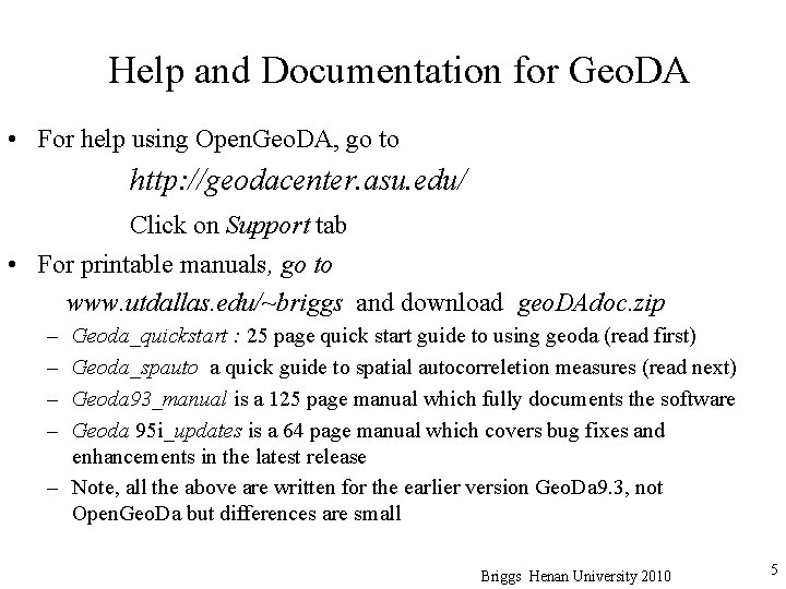
Help and Documentation for Geo. DA • For help using Open. Geo. DA, go to http: //geodacenter. asu. edu/ Click on Support tab • For printable manuals, go to www. utdallas. edu/~briggs and download geo. DAdoc. zip – – Geoda_quickstart : 25 page quick start guide to using geoda (read first) Geoda_spauto a quick guide to spatial autocorreletion measures (read next) Geoda 93_manual is a 125 page manual which fully documents the software Geoda 95 i_updates is a 64 page manual which covers bug fixes and enhancements in the latest release – Note, all the above are written for the earlier version Geo. Da 9. 3, not Open. Geo. Da but differences are small Briggs Henan University 2010 5

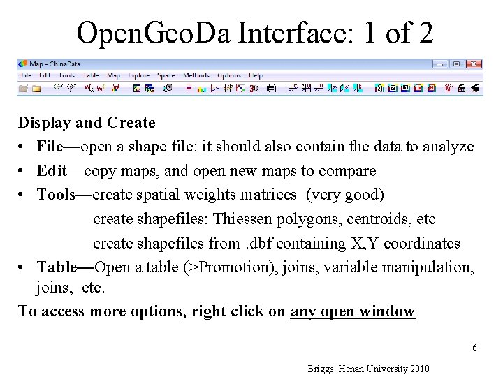
Open. Geo. Da Interface: 1 of 2 Display and Create • File—open a shape file: it should also contain the data to analyze • Edit—copy maps, and open new maps to compare • Tools—create spatial weights matrices (very good) create shapefiles: Thiessen polygons, centroids, etc create shapefiles from. dbf containing X, Y coordinates • Table—Open a table (>Promotion), joins, variable manipulation, joins, etc. To access more options, right click on any open window 6 Briggs Henan University 2010

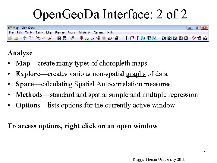
Open. Geo. Da Interface: 2 of 2 Analyze • Map—create many types of choropleth maps • Explore—creates various non-spatial graphs of data • Space—calculating Spatial Autocorrelation measures • Methods—standard and spatial simple and multiple regression • Options—lists options for the currently active window. To access options, right click on an open window 7 Briggs Henan University 2010

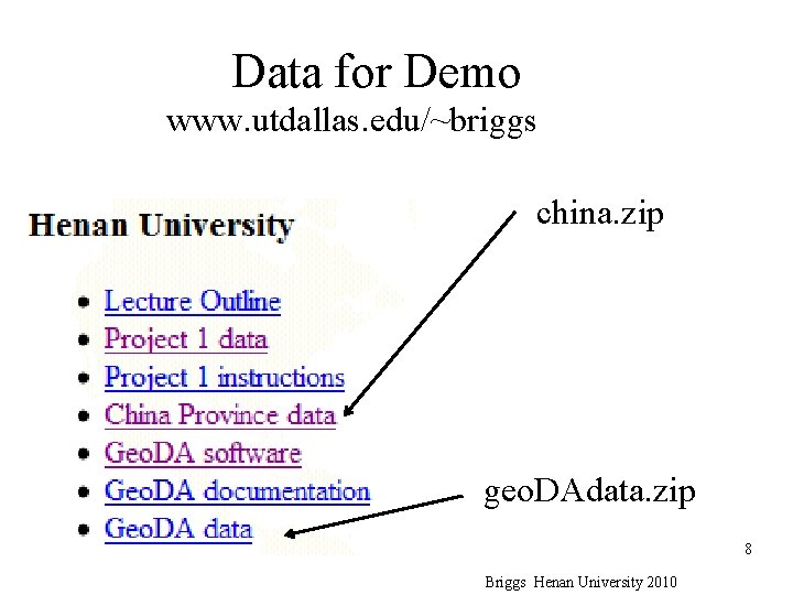
Data for Demo www. utdallas. edu/~briggs china. zip geo. DAdata. zip 8 Briggs Henan University 2010

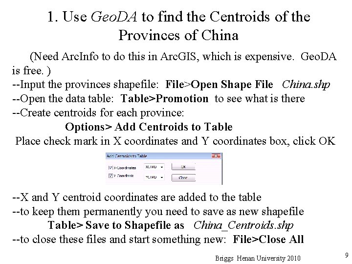
1. Use Geo. DA to find the Centroids of the Provinces of China (Need Arc. Info to do this in Arc. GIS, which is expensive. Geo. DA is free. ) --Input the provinces shapefile: File>Open Shape File China. shp --Open the data table: Table>Promotion to see what is there --Create centroids for each province: Options> Add Centroids to Table Place check mark in X coordinates and Y coordinates box, click OK --X and Y centroid coordinates are added to the table --to keep them permanently you need to save as new shapefile Table> Save to Shapefile as China_Centroids. shp --to close these files and start something new: File>Close All Briggs Henan University 2010 9

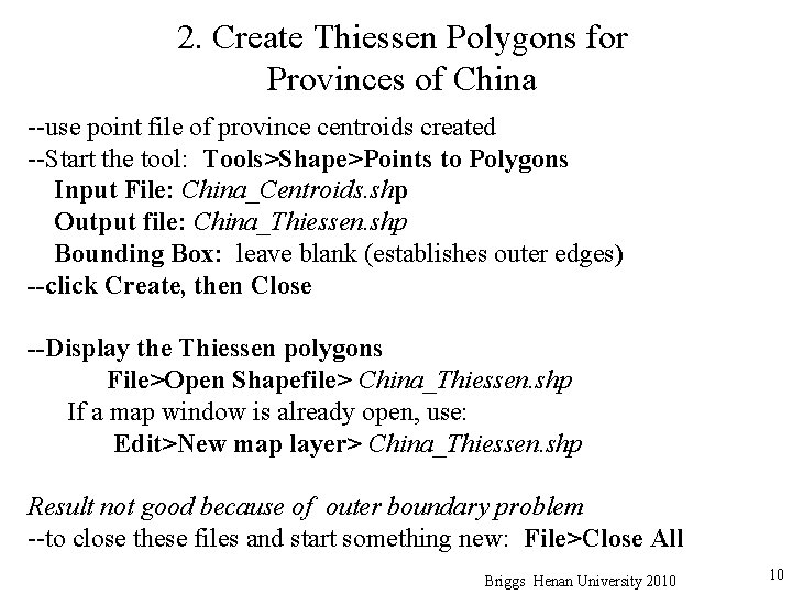
2. Create Thiessen Polygons for Provinces of China --use point file of province centroids created --Start the tool: Tools>Shape>Points to Polygons Input File: China_Centroids. shp Output file: China_Thiessen. shp Bounding Box: leave blank (establishes outer edges) --click Create, then Close --Display the Thiessen polygons File>Open Shapefile> China_Thiessen. shp If a map window is already open, use: Edit>New map layer> China_Thiessen. shp Result not good because of outer boundary problem --to close these files and start something new: File>Close All Briggs Henan University 2010 10

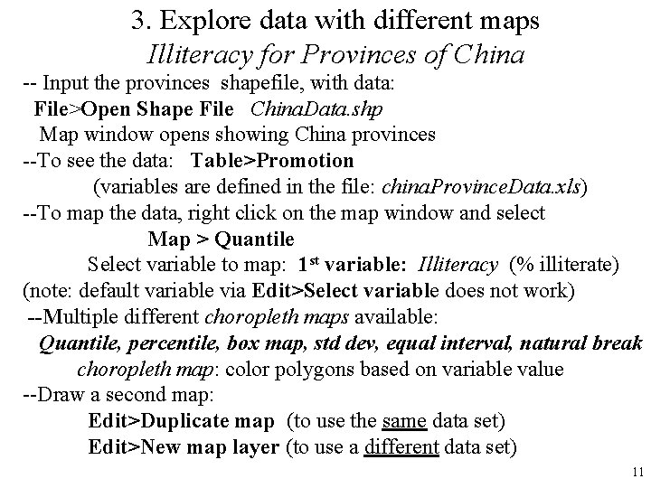
3. Explore data with different maps Illiteracy for Provinces of China -- Input the provinces shapefile, with data: File>Open Shape File China. Data. shp Map window opens showing China provinces --To see the data: Table>Promotion (variables are defined in the file: china. Province. Data. xls) --To map the data, right click on the map window and select Map > Quantile Select variable to map: 1 st variable: Illiteracy (% illiterate) (note: default variable via Edit>Select variable does not work) --Multiple different choropleth maps available: Quantile, percentile, box map, std dev, equal interval, natural break choropleth map: color polygons based on variable value --Draw a second map: Edit>Duplicate map (to use the same data set) Edit>New map layer (to use a different data set) 11

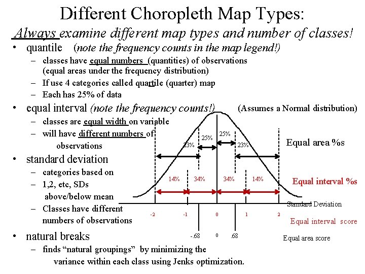
Different Choropleth Map Types: Always examine different map types and number of classes! • quantile (note the frequency counts in the map legend!) • – classes have equal numbers (quantities) of observations (equal areas under the frequency distribution) – If use 4 categories called quartile (quarter) map – Each has 25% of data (Assumes a Normal distribution) equal interval (note the frequency counts!) – classes are equal width on variable 25% – will have different numbers of 25% Equal area %s 23% observations • standard deviation – categories based on – 1, 2, etc, SDs above/below mean – Classes have different numbers of observations • natural breaks 14% 34% 14% Equal interval %s Standard Deviation -2 -1 0 -. 68 0 1 . 68 – finds “natural groupings” by minimizing the variance within each class using Jenks optimization. 2 Equal interval score Equal area score

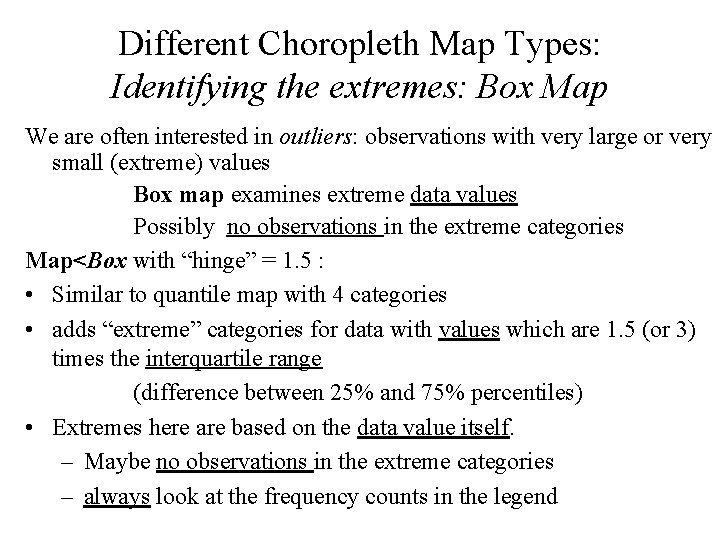
Different Choropleth Map Types: Identifying the extremes: Box Map We are often interested in outliers: observations with very large or very small (extreme) values Box map examines extreme data values Possibly no observations in the extreme categories Map<Box with “hinge” = 1. 5 : • Similar to quantile map with 4 categories • adds “extreme” categories for data with values which are 1. 5 (or 3) times the interquartile range (difference between 25% and 75% percentiles) • Extremes here are based on the data value itself. – Maybe no observations in the extreme categories – always look at the frequency counts in the legend

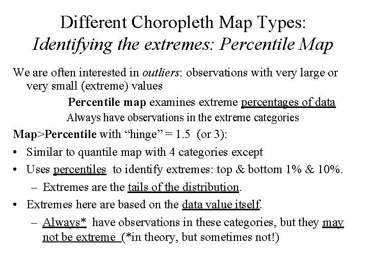
Different Choropleth Map Types: Identifying the extremes: Percentile Map We are often interested in outliers: observations with very large or very small (extreme) values Percentile map examines extreme percentages of data Always have observations in the extreme categories Map>Percentile with “hinge” = 1. 5 (or 3): • Similar to quantile map with 4 categories except • Uses percentiles to identify extremes: top & bottom 1% & 10%. – Extremes are the tails of the distribution. • Extremes here are based on the data value itself. – Always* have observations in these categories, but they may not be extreme (*in theory, but sometimes not!)

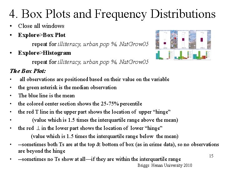
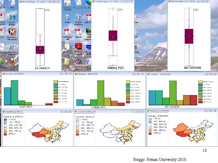
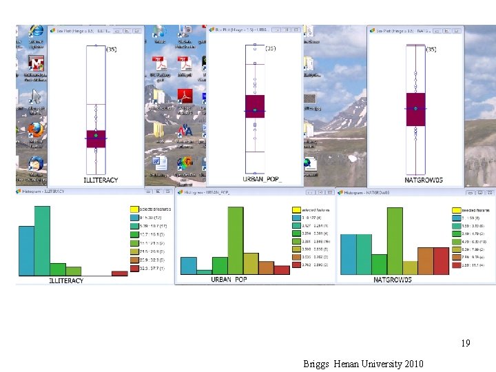
4. Box Plots and Frequency Distributions • Close all windows • Explore>Box Plot repeat for illiteracy, urban pop %, Nat. Grow 05 • Explore>Histogram repeat for illiteracy, urban pop %, Nat. Grow 05 The Box Plot: • all observations are positioned based on their value on the variable • the green asterisk is the median observation • The blue line is the mean • the colored center section shows the 25 -75% percentile • the red T line in the upper part shows the location of upper “hinge” • (value which is 1. 5 times the interquartile range above the mean) • the red in the lower part shows the location of lower “hinge” (value which is 1. 5 times the interquartile range below the mean) • --sometimes both Ts are at the top & bottom of box (as in crime data), so no observations are beyond the hinge 15 • --sometimes no Ts show at all—if they are within the interquartile range Briggs Henan University 2010

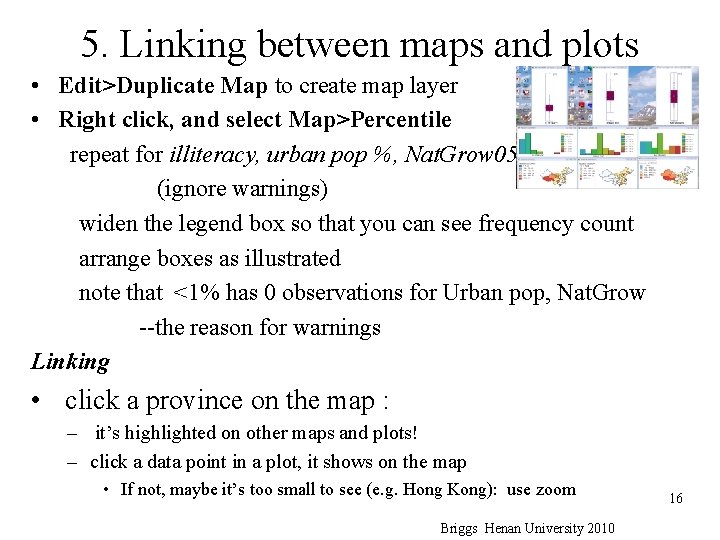
5. Linking between maps and plots • Edit>Duplicate Map to create map layer • Right click, and select Map>Percentile repeat for illiteracy, urban pop %, Nat. Grow 05 (ignore warnings) widen the legend box so that you can see frequency count arrange boxes as illustrated note that <1% has 0 observations for Urban pop, Nat. Grow --the reason for warnings Linking • click a province on the map : – it’s highlighted on other maps and plots! – click a data point in a plot, it shows on the map • If not, maybe it’s too small to see (e. g. Hong Kong): use zoom Briggs Henan University 2010 16

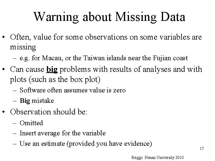
Warning about Missing Data • Often, value for some observations on some variables are missing – e. g. for Macau, or the Taiwan islands near the Fujian coast • Can cause big problems with results of analyses and with plots (such as the box plot) – Software often assumes value is zero – Big mistake • Observation should be: – Omitted – Insert average for the variable – Use an estimate (provided you have evidence) Briggs Henan University 2010 17

18 Briggs Henan University 2010

19 Briggs Henan University 2010

6. Moran’s I and Lisa 20 Briggs Henan University 2010

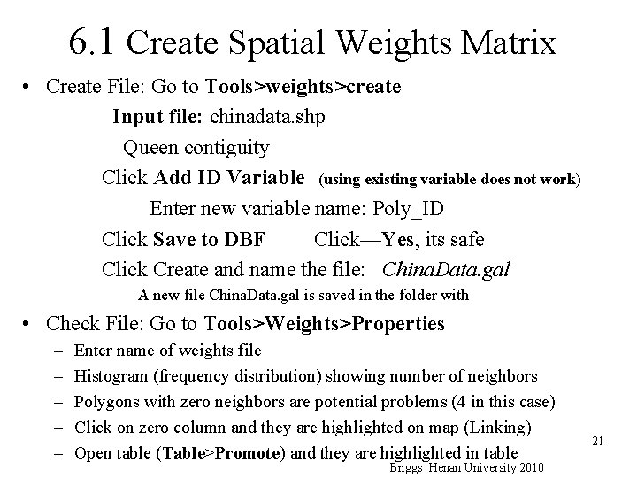
6. 1 Create Spatial Weights Matrix • Create File: Go to Tools>weights>create Input file: chinadata. shp Queen contiguity Click Add ID Variable (using existing variable does not work) Enter new variable name: Poly_ID Click Save to DBF Click—Yes, its safe Click Create and name the file: China. Data. gal A new file China. Data. gal is saved in the folder with • Check File: Go to Tools>Weights>Properties – – – Enter name of weights file Histogram (frequency distribution) showing number of neighbors Polygons with zero neighbors are potential problems (4 in this case) Click on zero column and they are highlighted on map (Linking) Open table (Table>Promote) and they are highlighted in table Briggs Henan University 2010 21

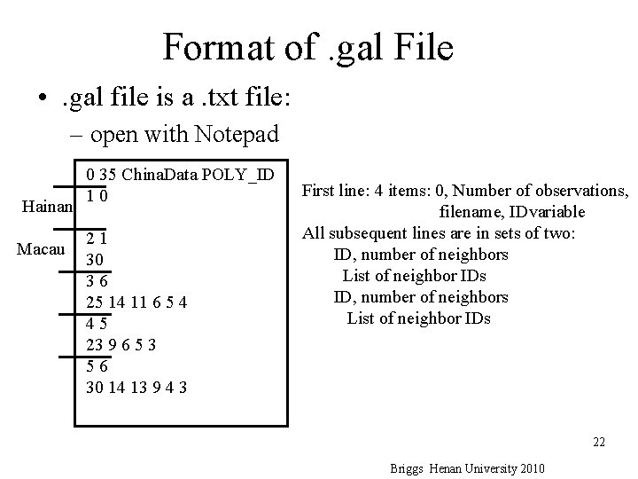
Format of. gal File • . gal file is a. txt file: – open with Notepad Hainan Macau 0 35 China. Data POLY_ID 1 0 2 1 30 3 6 25 14 11 6 5 4 4 5 23 9 6 5 3 5 6 30 14 13 9 4 3 First line: 4 items: 0, Number of observations, filename, IDvariable All subsequent lines are in sets of two: ID, number of neighbors List of neighbor IDs 22 Briggs Henan University 2010

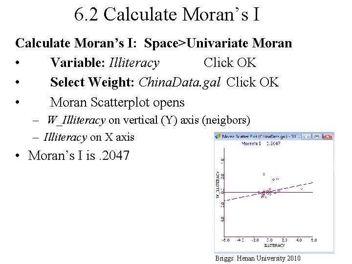
6. 2 Calculate Moran’s I: Space>Univariate Moran • Variable: Illiteracy Click OK • Select Weight: China. Data. gal Click OK • Moran Scatterplot opens – W_Illiteracy on vertical (Y) axis (neigbors) – Illiteracy on X axis • Moran’s I is. 2047 23 Briggs Henan University 2010

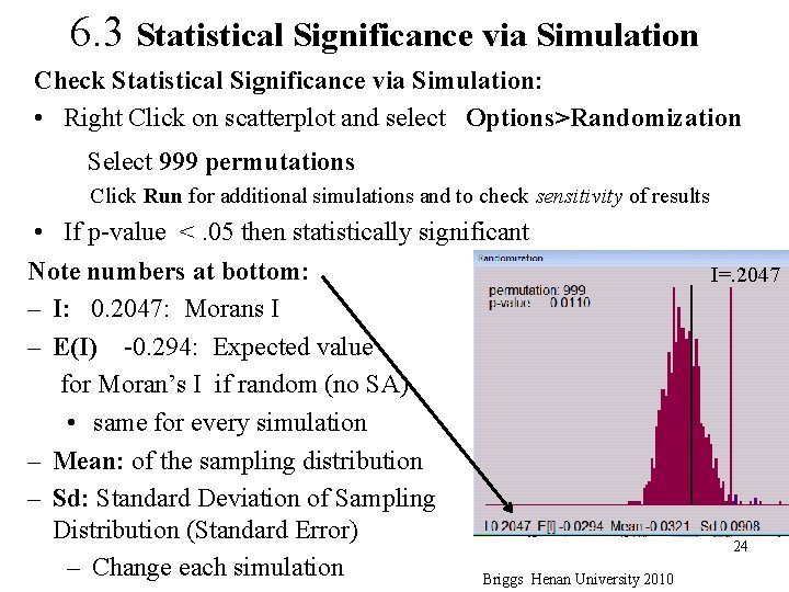
6. 3 Statistical Significance via Simulation Check Statistical Significance via Simulation: • Right Click on scatterplot and select Options>Randomization Select 999 permutations Click Run for additional simulations and to check sensitivity of results • If p-value <. 05 then statistically significant Note numbers at bottom: – I: 0. 2047: Morans I – E(I) -0. 294: Expected value for Moran’s I if random (no SA) • same for every simulation – Mean: of the sampling distribution – Sd: Standard Deviation of Sampling Distribution (Standard Error) – Change each simulation Briggs Henan University 2010 I=. 2047 24

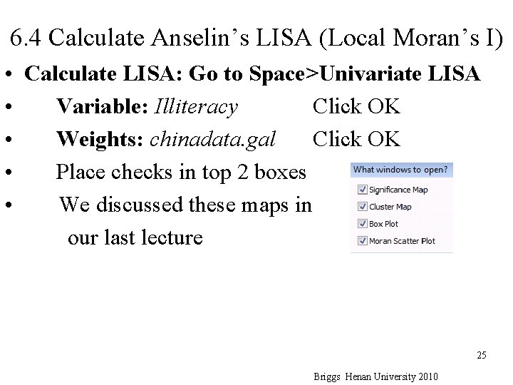
6. 4 Calculate Anselin’s LISA (Local Moran’s I) • Calculate LISA: Go to Space>Univariate LISA • Variable: Illiteracy Click OK • Weights: chinadata. gal Click OK • Place checks in top 2 boxes • We discussed these maps in our last lecture 25 Briggs Henan University 2010

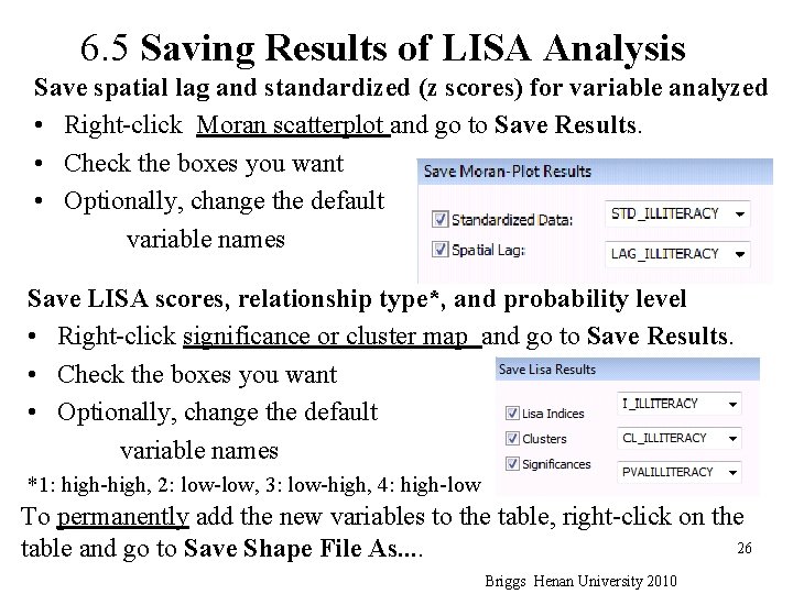
6. 5 Saving Results of LISA Analysis Save spatial lag and standardized (z scores) for variable analyzed • Right-click Moran scatterplot and go to Save Results. • Check the boxes you want • Optionally, change the default variable names Save LISA scores, relationship type*, and probability level • Right-click significance or cluster map and go to Save Results. • Check the boxes you want • Optionally, change the default variable names *1: high-high, 2: low-low, 3: low-high, 4: high-low To permanently add the new variables to the table, right-click on the 26 table and go to Save Shape File As. . Briggs Henan University 2010

6. 6 Recomputing Moran’s I for selected observations The Moran's I slope and value can be recomputed for all observations excluding the ones selected: • Right-click on Moran scatterplot and choose Exclude Selected Exclude selected observations • Click an individual observation or drag a box and Moran’s I is recomputed excluding selected observation(s) – New value shown in red on top right – Exclude observations also highlighted on maps Exclude groups of observation by brushing • Hold Ctrl key and draw a rectangle; release mouse, then release Ctrl key; rectangle flashes; • Use mouse to move rectangle across screen • Moran’s I recalculated excluding observations within rectangle Note: not a true Moran's I since lag-X not adjusted for excluded observations. Briggs Henan University 2010 27

Hints on getting your data into geoda • Data (variables) must be in a shapefile, or in a. dbf which you join to the shapefile using Table>Join tables • a shapefile also stores data in a. dbf file which you can edit to add variables How do I edit a. dbf file to add data? • Use Excel 2003 or earlier – You can save files from Excel in. dbf format – Excel 2007 or later will read but not write. dbf files • Use Open. Office from Sun/Oracle www. openoffice. org An almost exact replica of Excel which is free Briggs Henan University 2010 28

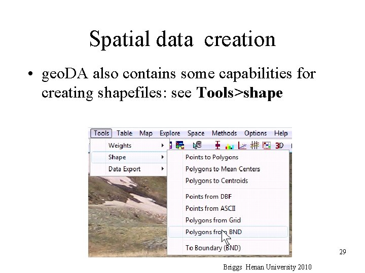
Spatial data creation • geo. DA also contains some capabilities for creating shapefiles: see Tools>shape 29 Briggs Henan University 2010

What have we learned today? How to use geo. DA for • general exploration of spatial data • analysis of spatial autocorrelation Next time • spatial regression • Then, using geo. DA for spatial regression 30 Briggs Henan University 2010