Using Alloy to model an algorithm that finds


![Prim’s algorithm • Prim’s algorithm is a step-by-step procedure for finding paths [1] from Prim’s algorithm • Prim’s algorithm is a step-by-step procedure for finding paths [1] from](https://slidetodoc.com/presentation_image/58527a0c02aaabfdf71c56ac9909db11/image-9.jpg)
![Time T 0 T 1 … Alloy code: open util/ordering[Time] Node sig Time {} Time T 0 T 1 … Alloy code: open util/ordering[Time] Node sig Time {}](https://slidetodoc.com/presentation_image/58527a0c02aaabfdf71c56ac9909db11/image-31.jpg)
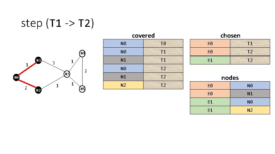
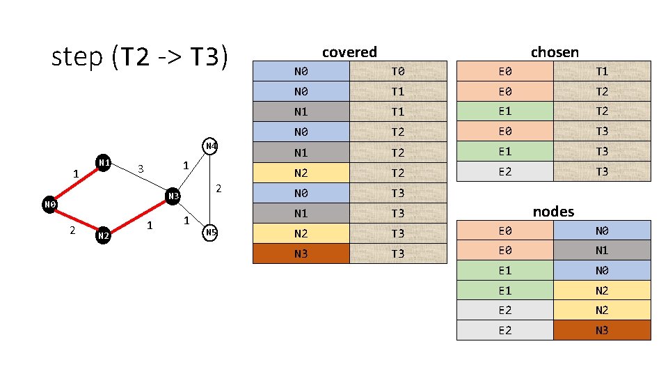
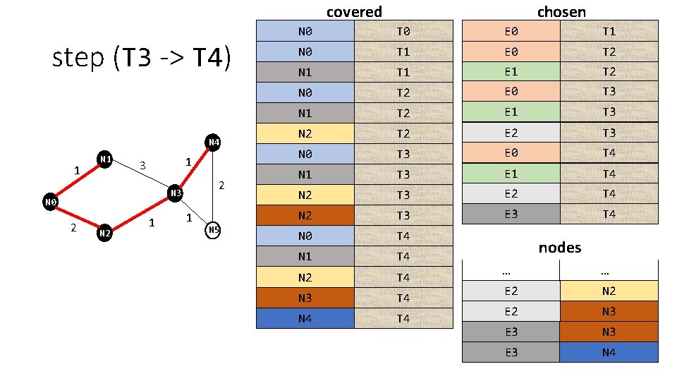
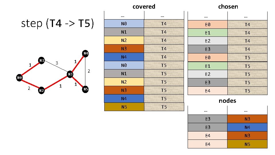

![new edge Nodes covered nodes cutting[e, t] new edge Nodes covered nodes cutting[e, t]](https://slidetodoc.com/presentation_image/58527a0c02aaabfdf71c56ac9909db11/image-73.jpg)
![new edge Nodes W=1 covered nodes W=2 w=2 (cutting[e, t] and (no e 2: new edge Nodes W=1 covered nodes W=2 w=2 (cutting[e, t] and (no e 2:](https://slidetodoc.com/presentation_image/58527a0c02aaabfdf71c56ac9909db11/image-74.jpg)
![open util/ordering[Time] sig Time {} sig Node {covered: set Time} sig Edge {weight: Int, open util/ordering[Time] sig Time {} sig Node {covered: set Time} sig Edge {weight: Int,](https://slidetodoc.com/presentation_image/58527a0c02aaabfdf71c56ac9909db11/image-81.jpg)
![prim(graph *g, int start) { int i; edgenode *p; bool intree[MAXV+1]; int distance[MAXV+1] int prim(graph *g, int start) { int i; edgenode *p; bool intree[MAXV+1]; int distance[MAXV+1] int](https://slidetodoc.com/presentation_image/58527a0c02aaabfdf71c56ac9909db11/image-83.jpg)
![correct: check { spanning. Tree [chosen. last] } for 5 but 10 Edge, 5 correct: check { spanning. Tree [chosen. last] } for 5 but 10 Edge, 5](https://slidetodoc.com/presentation_image/58527a0c02aaabfdf71c56ac9909db11/image-110.jpg)



- Slides: 117

Using Alloy to model an algorithm that finds the shortest path between nodes Roger L. Costello December 29, 2016

Acknowledgement The model shown in these slides comes from this (fantastic) paper. http: //sdg. csail. mit. edu/pubs/2012/abz 12 -overflow. pdf

Special thanks • Special thanks to Aleksandar Milicevic for reviewing this slide deck and identifying all the places that I messed up. Thanks Aleksandar!

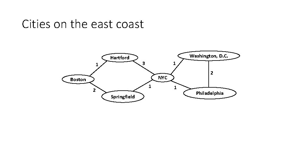
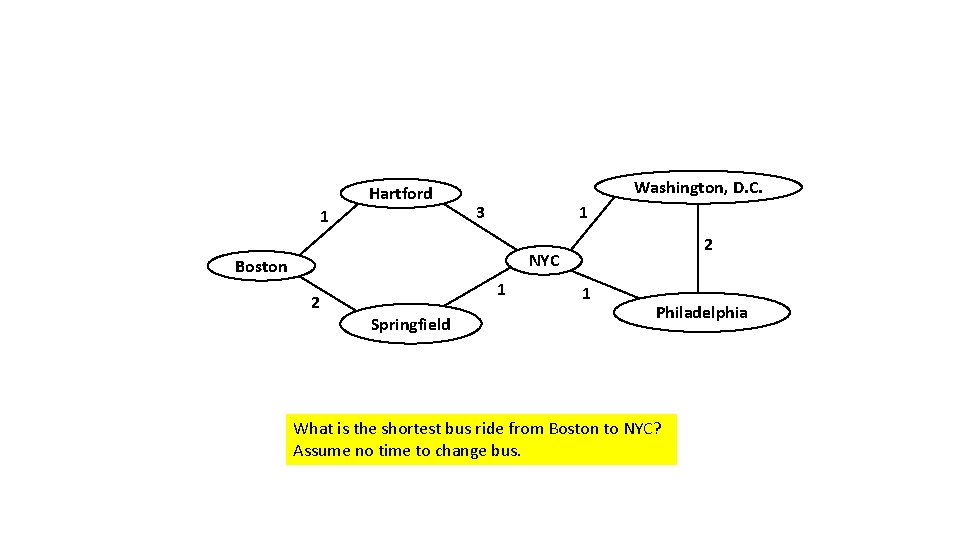
Cities on the east coast Hartford 1 Washington, D. C. 3 1 2 NYC Boston 2 1 Springfield 1 Philadelphia

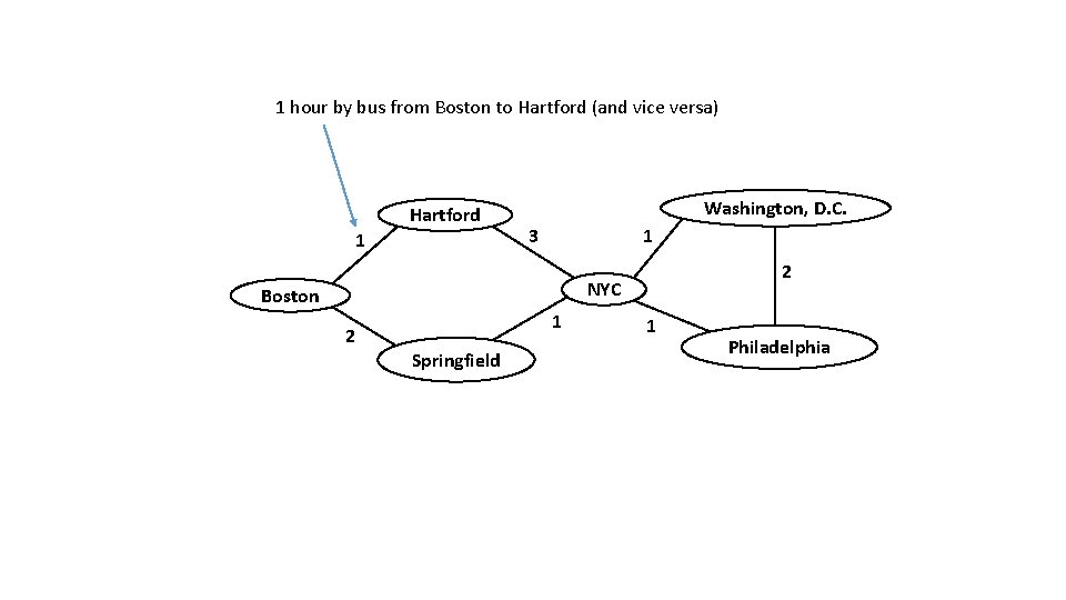
1 hour by bus from Boston to Hartford (and vice versa) Hartford 1 Washington, D. C. 3 1 2 NYC Boston 2 1 Springfield 1 Philadelphia

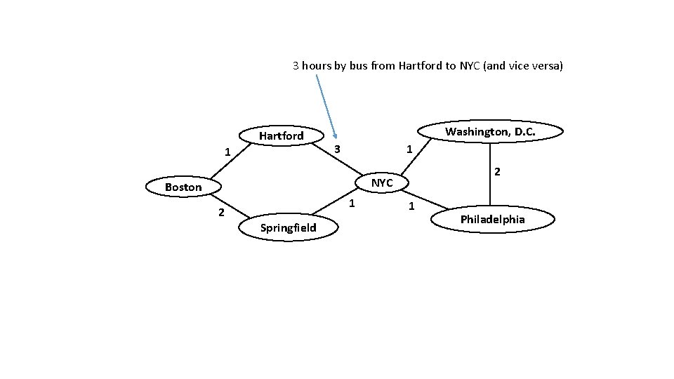
3 hours by bus from Hartford to NYC (and vice versa) Hartford 1 Washington, D. C. 3 1 2 NYC Boston 2 1 Springfield 1 Philadelphia

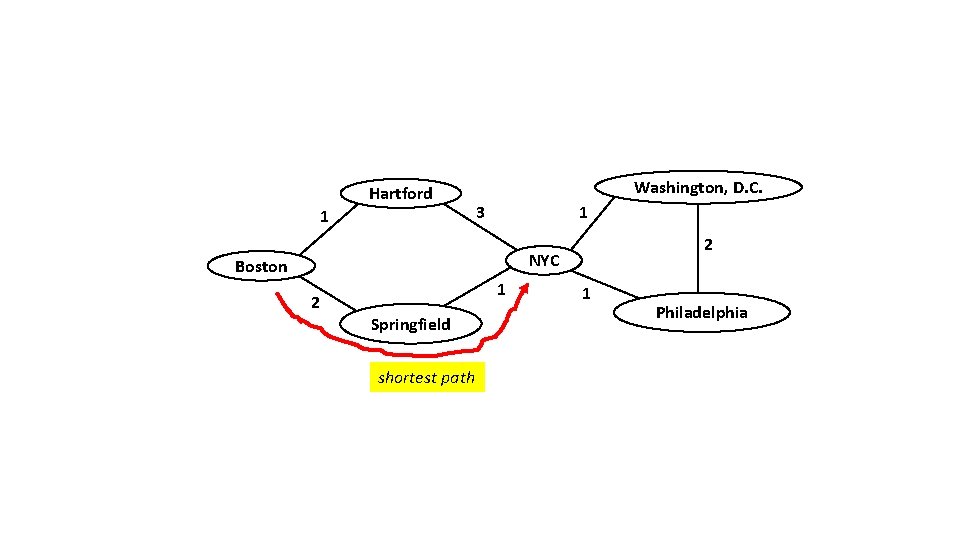
Hartford 1 Washington, D. C. 3 1 2 NYC Boston 2 1 Springfield 1 Philadelphia What is the shortest bus ride from Boston to NYC? Assume no time to change bus.

Hartford 1 Washington, D. C. 3 1 2 NYC Boston 2 1 Springfield shortest path 1 Philadelphia
![Prims algorithm Prims algorithm is a stepbystep procedure for finding paths 1 from Prim’s algorithm • Prim’s algorithm is a step-by-step procedure for finding paths [1] from](https://slidetodoc.com/presentation_image/58527a0c02aaabfdf71c56ac9909db11/image-9.jpg)
Prim’s algorithm • Prim’s algorithm is a step-by-step procedure for finding paths [1] from one city to any other city (more generically, from one node to any other node). • Let’s take an example to illustrate Prim’s algorithm. [1] Actually, Prim’s algorithm finds a minimum spanning tree (MST), not a "shortest path from one node to any other node". We’ll talk about spanning trees later. For now, just think of Prim as finding a short path from A to B.

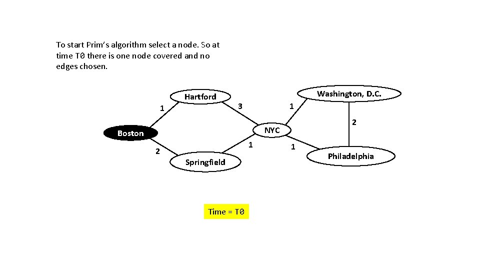
To start Prim’s algorithm select a node. So at time T 0 there is one node covered and no edges chosen. Hartford 1 Washington, D. C. 3 1 2 NYC Boston 2 1 Springfield Time = T 0 1 Philadelphia

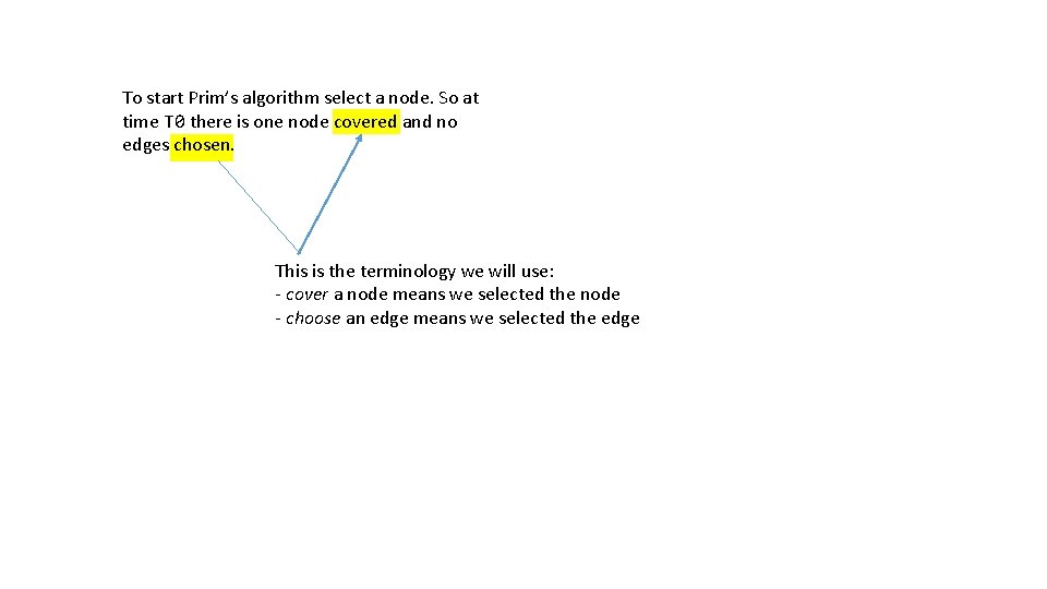
To start Prim’s algorithm select a node. So at time T 0 there is one node covered and no edges chosen. This is the terminology we will use: - cover a node means we selected the node - choose an edge means we selected the edge

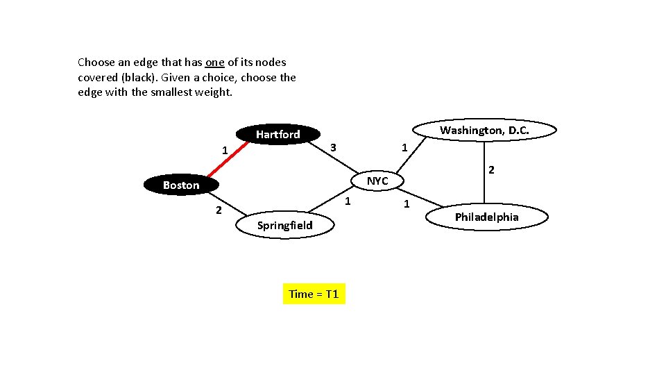
Choose an edge that has one of its nodes covered (black). Given a choice, choose the edge with the smallest weight. Hartford 1 Washington, D. C. 3 1 2 NYC Boston 2 1 Springfield Time = T 1 1 Philadelphia

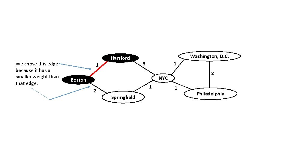
We chose this edge because it has a smaller weight than that edge. Hartford 1 Washington, D. C. 3 1 2 NYC Boston 2 1 Springfield 1 Philadelphia

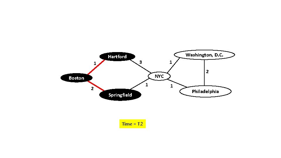
Hartford 1 Washington, D. C. 3 1 2 NYC Boston 2 1 Springfield Time = T 2 1 Philadelphia

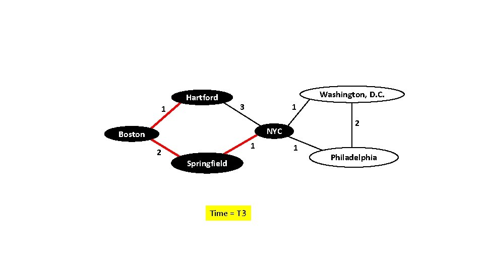
Hartford 1 Washington, D. C. 3 1 2 NYC Boston 2 1 Springfield Time = T 3 1 Philadelphia

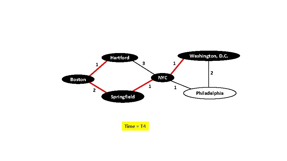
Hartford 1 Washington, D. C. 3 1 2 NYC Boston 2 1 Springfield Time = T 4 1 Philadelphia

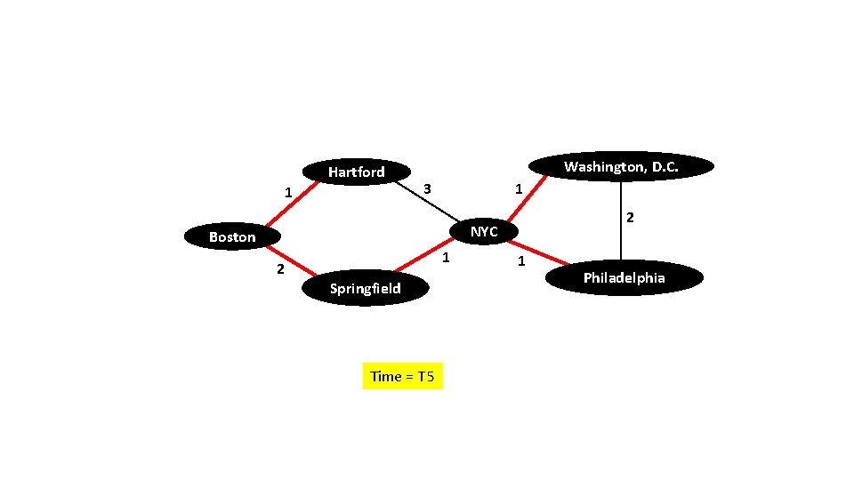
Hartford 1 Washington, D. C. 3 1 2 NYC Boston 2 1 Springfield Time = T 5 1 Philadelphia

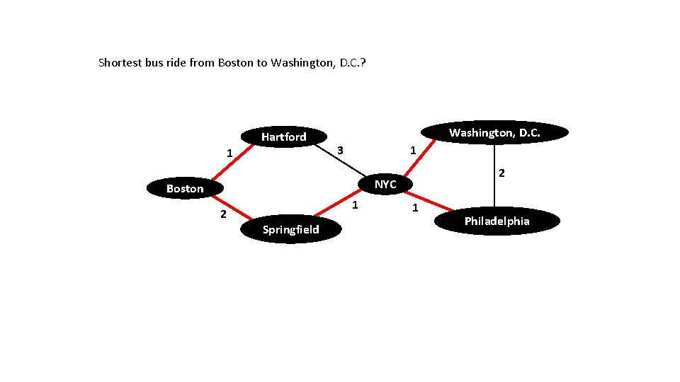
Shortest bus ride from Boston to Washington, D. C. ? Hartford 1 Washington, D. C. 3 1 2 NYC Boston 2 1 Springfield 1 Philadelphia

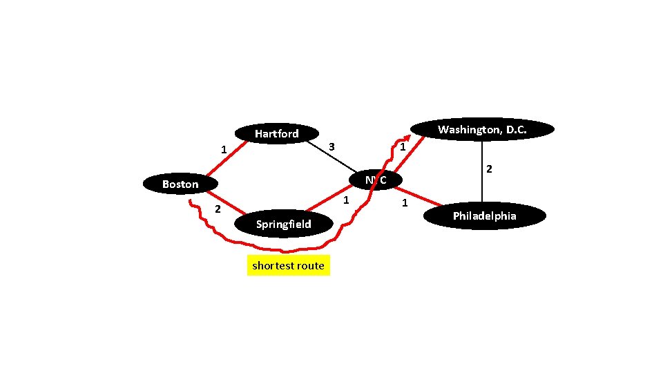
Hartford 1 Washington, D. C. 3 1 2 NYC Boston 2 1 Springfield shortest route 1 Philadelphia

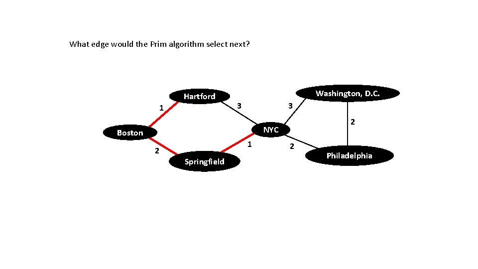
What edge would the Prim algorithm select next? Hartford 1 Washington, D. C. 3 3 2 NYC Boston 2 1 Springfield 2 Philadelphia

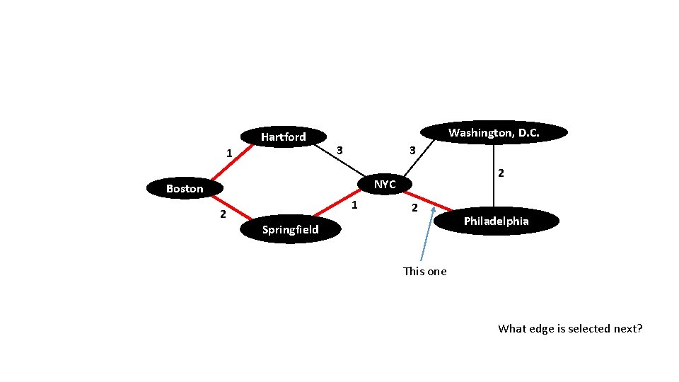
Hartford 1 Washington, D. C. 3 3 2 NYC Boston 2 1 2 Springfield Philadelphia This one What edge is selected next?

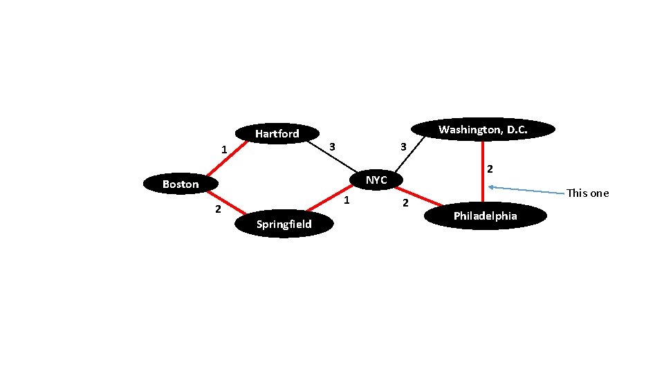
Hartford 1 Washington, D. C. 3 3 2 NYC Boston 2 1 Springfield 2 This one Philadelphia

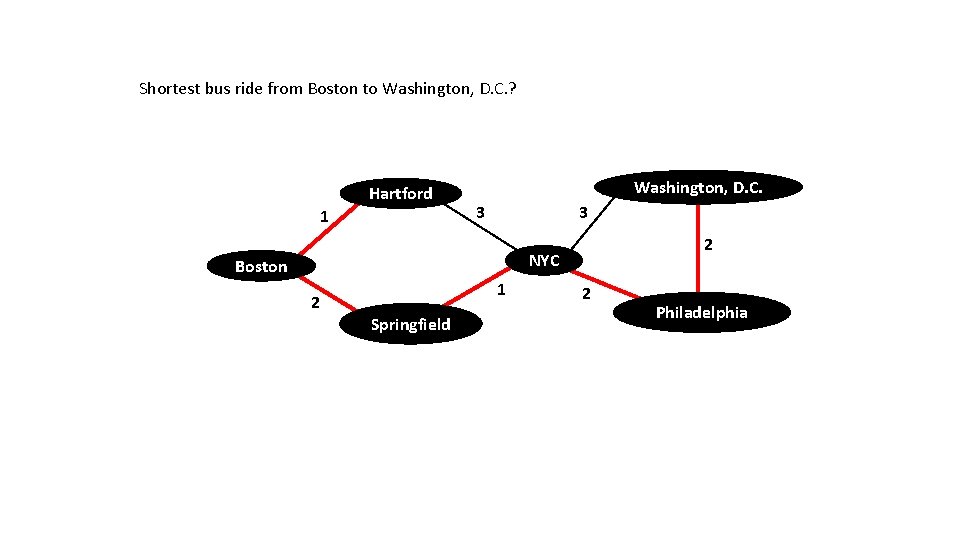
Shortest bus ride from Boston to Washington, D. C. ? Hartford 1 Washington, D. C. 3 3 2 NYC Boston 2 1 Springfield 2 Philadelphia

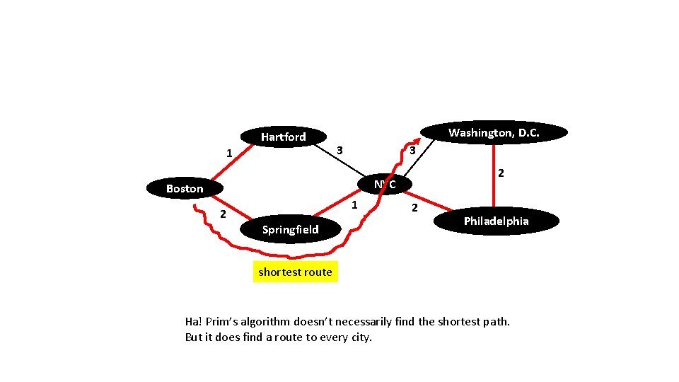
Hartford 1 Washington, D. C. 3 3 2 NYC Boston 2 1 Springfield 2 Philadelphia shortest route Ha! Prim’s algorithm doesn’t necessarily find the shortest path. But it does find a route to every city.

That illustrates the Prim algorithm. Now let’s model the Prim algorithm.

But first, what’s the goal of the model? • Whenever you create a model, you do so for a reason. In this case, we want to see if the Prim algorithm satisfies something. • What should the Prim algorithm satisfy? • The Prim algorithm should allow one to traverse from one node to any other node.

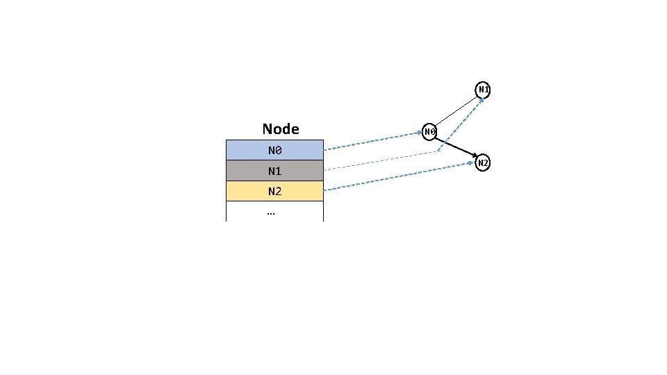
Nodes (rather than cities) • On the previous slides we showed the Prim algorithm in action on a graph of cities. • The Prim algorithm works on any graph, not just cities. • Let’s abstract the graph and refer to each junction in the graph as a “node. ” • So, the first thing we need to model is the set of nodes.

N 1 Node N 0 N 1 N 2 … N 0 N 2

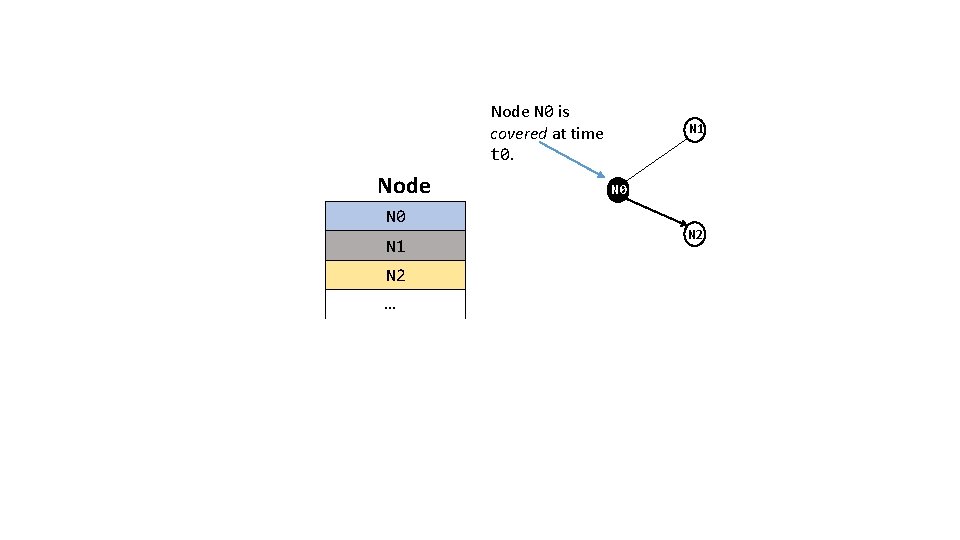
Node N 0 is covered at time t 0. Node N 0 N 1 N 2 … N 1 N 0 N 2

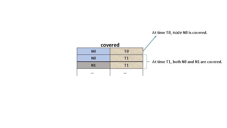
At time T 0, node N 0 is covered N 0 T 0 N 0 T 1 N 1 T 1 … … At time T 1, both N 0 and N 1 are covered.
![Time T 0 T 1 Alloy code open utilorderingTime Node sig Time Time T 0 T 1 … Alloy code: open util/ordering[Time] Node sig Time {}](https://slidetodoc.com/presentation_image/58527a0c02aaabfdf71c56ac9909db11/image-31.jpg)
Time T 0 T 1 … Alloy code: open util/ordering[Time] Node sig Time {} N 0 N 1 sig Node {covered: set Time} N 2 … covered N 0 T 0 N 0 T 1 N 1 T 1 … …

The second basic component • Graphs have nodes. We just modeled them. • Graphs also have edges, which we model next.

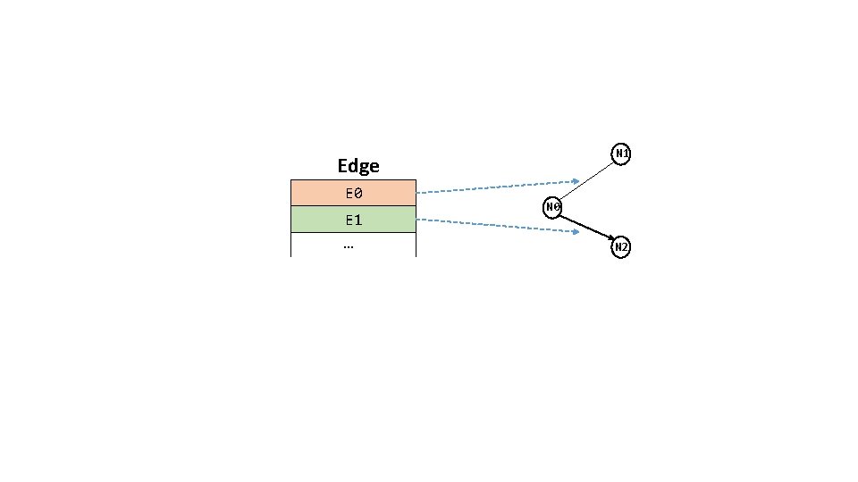
N 1 Edge E 0 E 1 … N 0 N 2

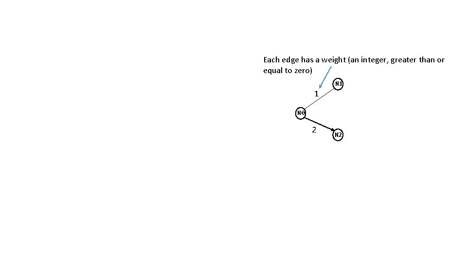
Each edge has a weight (an integer, greater than or equal to zero) N 1 1 N 0 2 N 2

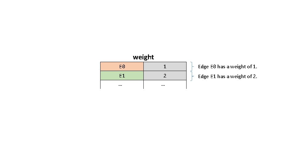
weight E 0 1 Edge E 0 has a weight of 1. E 1 2 Edge E 1 has a weight of 2. … …

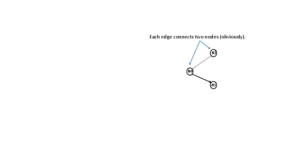
Each edge connects two nodes (obviously). N 2 N 0 N 1

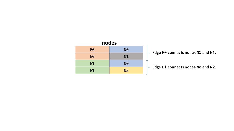
nodes E 0 N 0 E 0 N 1 E 1 N 0 E 1 N 2 Edge E 0 connects nodes N 0 and N 1. Edge E 1 connects nodes N 0 and N 2.

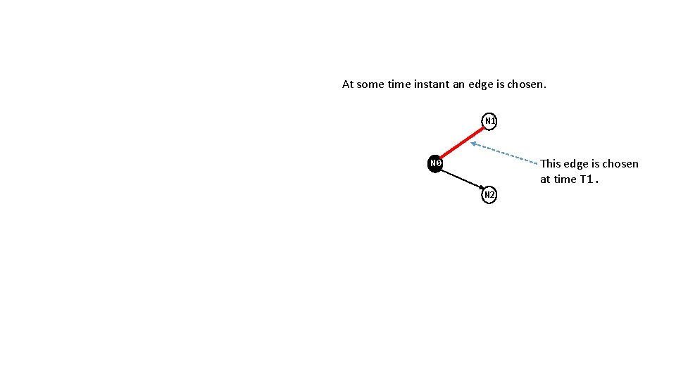
At some time instant an edge is chosen. N 1 This edge is chosen at time T 1. N 0 N 2

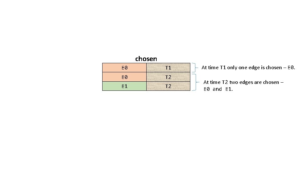
chosen E 0 T 1 E 0 T 2 E 1 T 2 At time T 1 only one edge is chosen – E 0. At time T 2 two edges are chosen – E 0 and E 1.

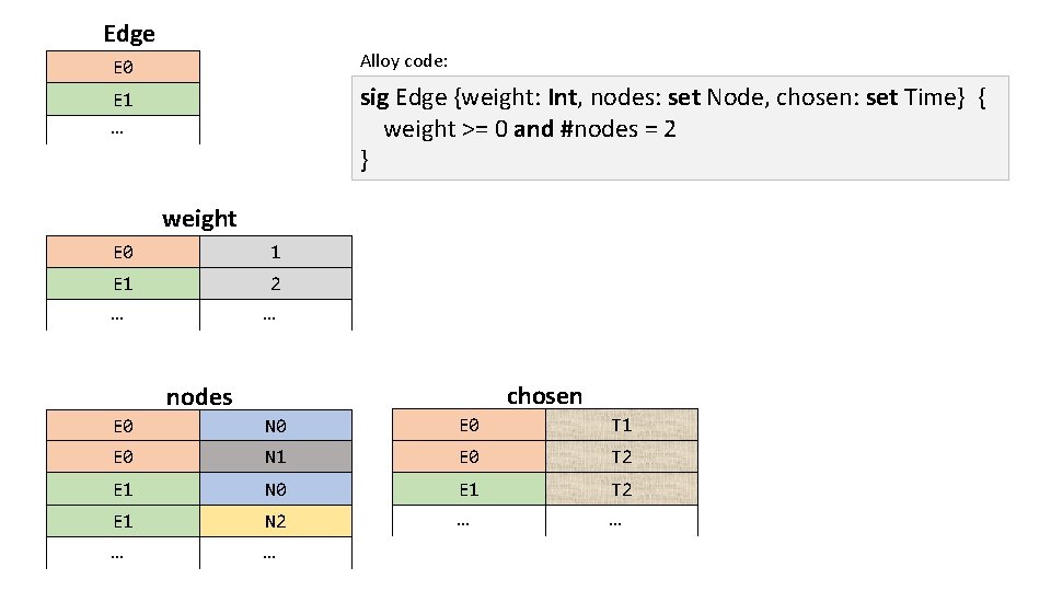
Edge E 0 Alloy code: E 1 … sig Edge {weight: Int, nodes: set Node, chosen: set Time} { weight >= 0 and #nodes = 2 } weight E 0 1 E 1 … 2 … chosen nodes E 0 N 0 E 0 T 1 E 0 N 1 E 0 T 2 E 1 N 0 E 1 T 2 E 1 N 2 … …

We’ve modeled the structural components (nodes, edges) and their relations (covered, weight, nodes, chosen). Now let’s model the operations in the Prim algorithm.

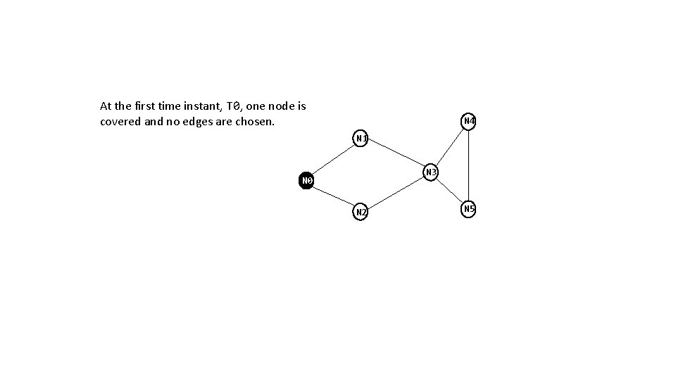
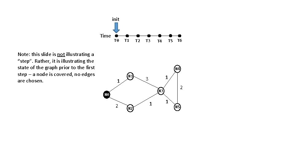
At the first time instant, T 0, one node is covered and no edges are chosen. N 4 N 1 N 3 N 0 N 2 N 5

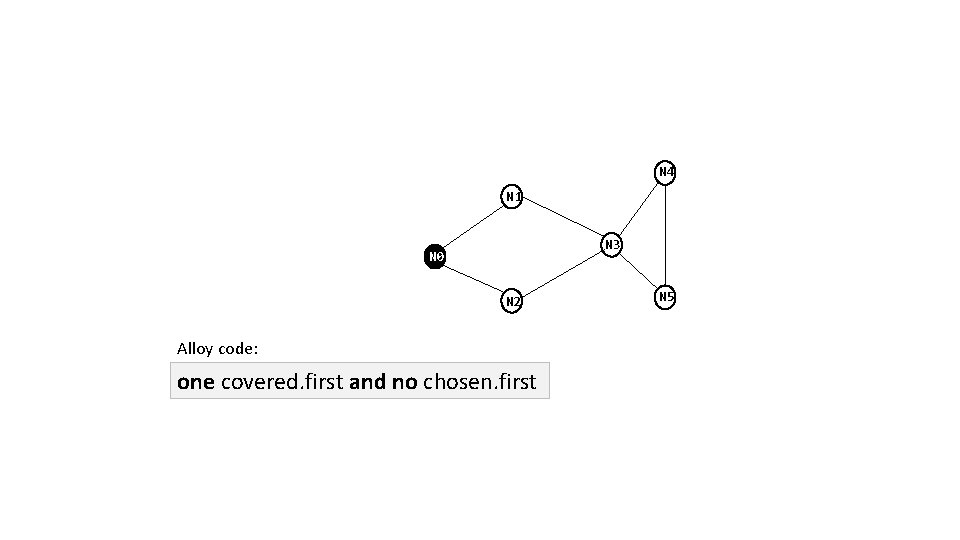
N 4 N 1 N 3 N 0 N 2 Alloy code: one covered. first and no chosen. first N 5

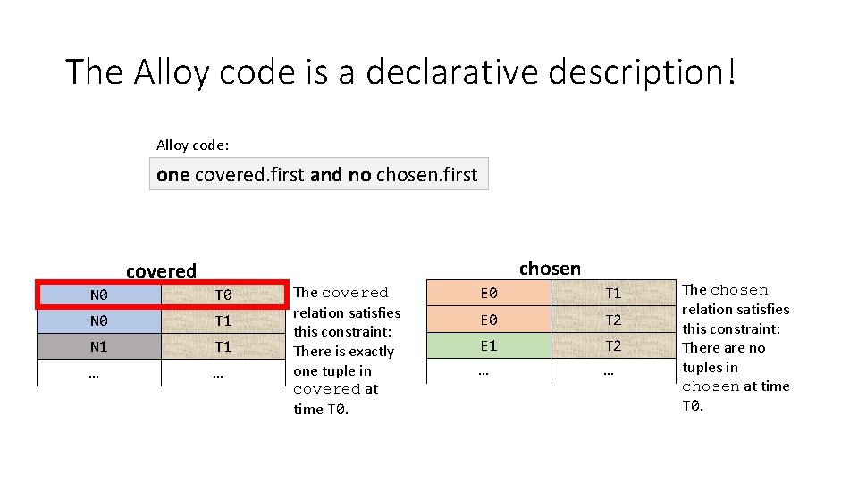
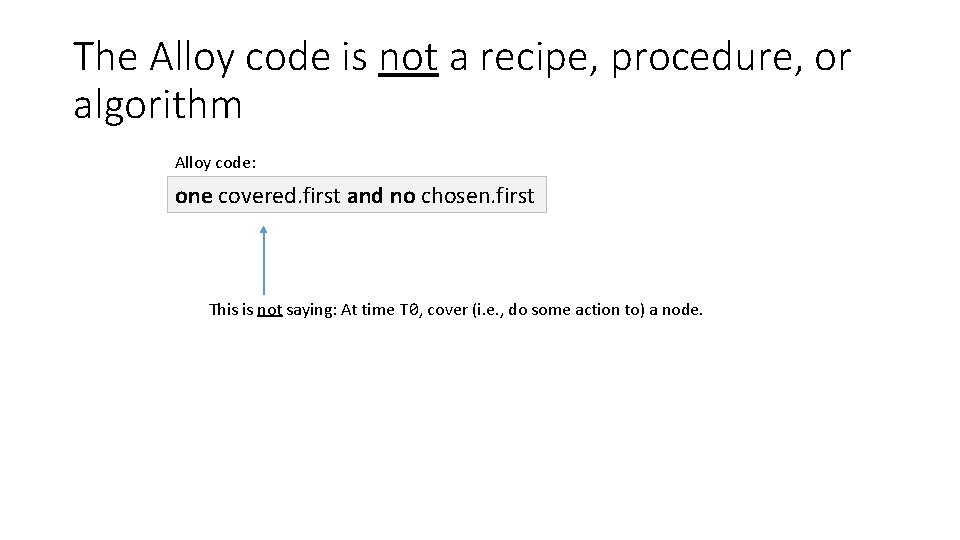
The Alloy code is a declarative description! Alloy code: one covered. first and no chosen. first chosen covered N 0 T 0 N 0 T 1 N 1 T 1 … … The covered relation satisfies this constraint: There is exactly one tuple in covered at time T 0. E 0 T 1 E 0 T 2 E 1 T 2 … … The chosen relation satisfies this constraint: There are no tuples in chosen at time T 0.

The Alloy code is not a recipe, procedure, or algorithm Alloy code: one covered. first and no chosen. first This is not saying: At time T 0, cover (i. e. , do some action to) a node.

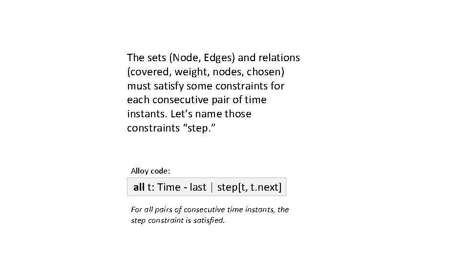
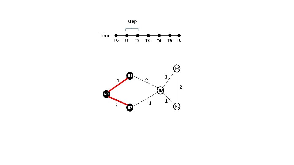
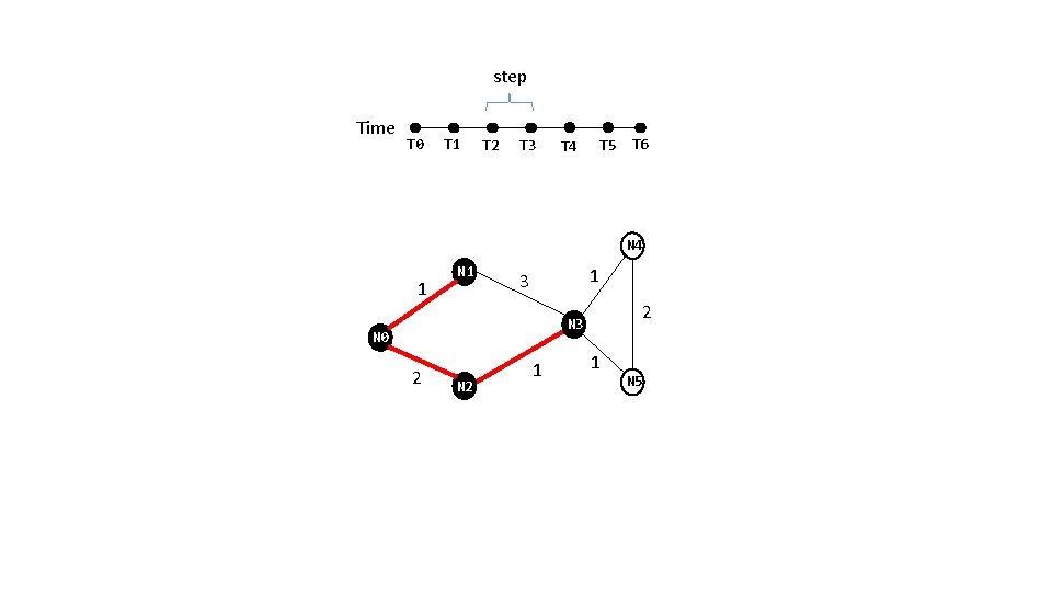
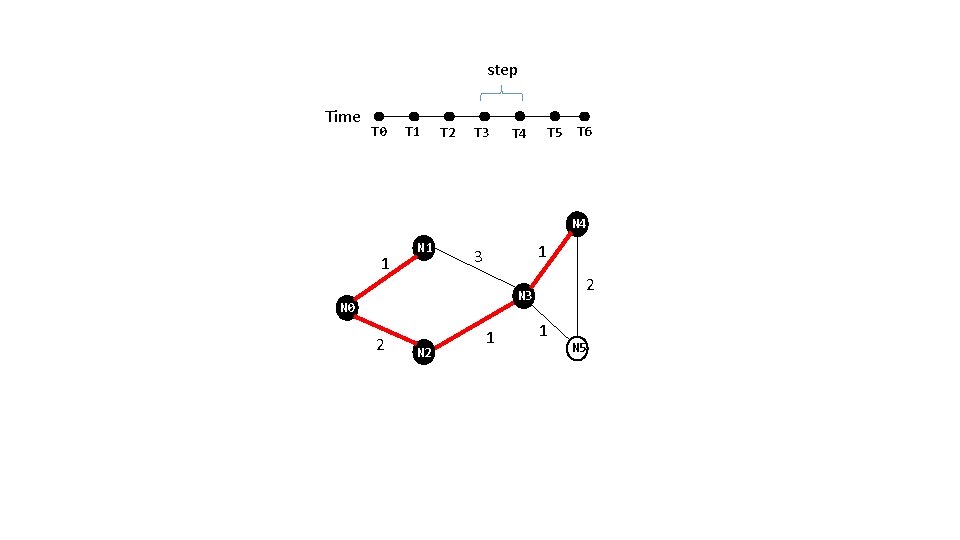
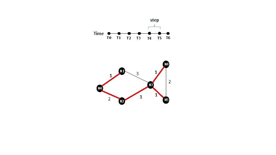
The sets (Node, Edges) and relations (covered, weight, nodes, chosen) must satisfy some constraints for each consecutive pair of time instants. Let’s name those constraints “step. ” Alloy code: all t: Time - last | step[t, t. next] For all pairs of consecutive time instants, the step constraint is satisfied.

init Time Note: this slide is not illustrating a “step”. Rather, it is illustrating the state of the graph prior to the first step – a node is covered, no edges are chosen. T 0 T 1 T 2 T 3 T 4 T 5 T 6 N 4 1 N 1 1 3 2 N 3 N 0 2 N 2 1 1 N 5

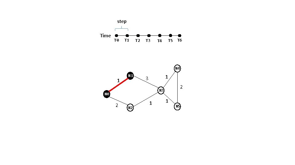
step Time T 0 T 1 T 2 T 3 T 4 T 5 T 6 N 4 1 N 1 1 3 2 N 3 N 0 2 N 2 1 1 N 5

step Time T 0 T 1 T 2 T 3 T 4 T 5 T 6 N 4 1 N 1 1 3 2 N 3 N 0 2 N 2 1 1 N 5

step Time T 0 T 1 T 2 T 3 T 4 T 5 T 6 N 4 1 N 1 1 3 2 N 3 N 0 2 N 2 1 1 N 5

step Time T 0 T 1 T 2 T 3 T 4 T 5 T 6 N 4 1 N 1 1 3 2 N 3 N 0 2 N 2 1 1 N 5

step Time T 0 T 1 T 2 T 3 T 4 T 5 T 6 N 4 1 N 1 1 3 2 N 3 N 0 2 N 2 1 1 N 5

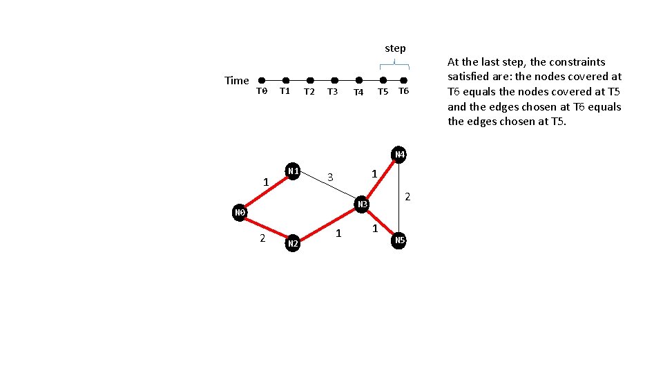
step Time T 0 T 1 T 2 T 3 T 4 T 5 T 6 N 4 1 N 1 1 3 2 N 3 N 0 2 N 2 1 1 N 5 At the last step, the constraints satisfied are: the nodes covered at T 6 equals the nodes covered at T 5 and the edges chosen at T 6 equals the edges chosen at T 5.

Let’s go through that again, this time showing the covered, chosen, and nodes relations.

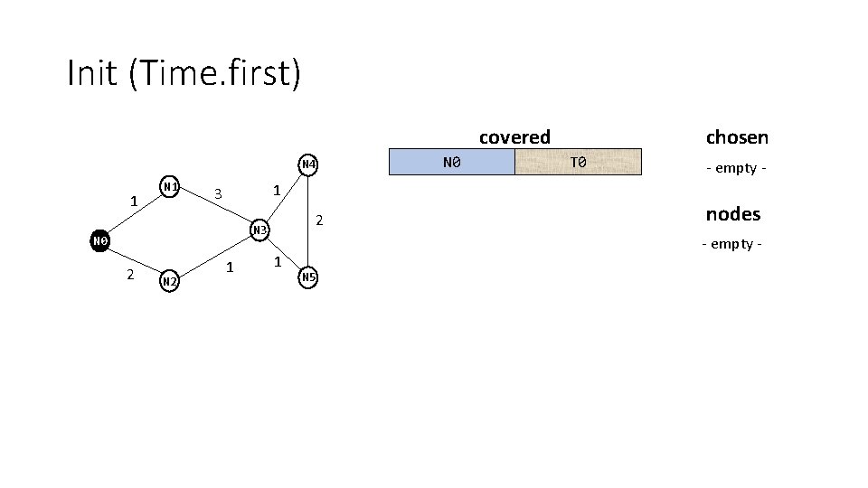
Init (Time. first) covered N 4 1 N 0 N 2 T 0 - empty - 1 3 2 N 0 chosen 1 1 nodes - empty - N 5

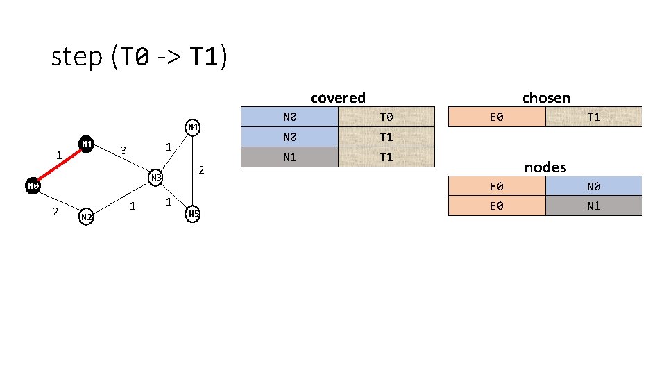
step (T 0 -> T 1) covered N 4 1 N 1 1 3 2 N 3 N 0 2 N 2 1 1 N 5 chosen N 0 T 0 N 0 T 1 N 1 T 1 E 0 T 1 nodes E 0 N 0 E 0 N 1

step (T 1 -> T 2) covered N 4 1 N 1 1 3 2 N 3 N 0 2 N 2 1 1 N 5 chosen N 0 T 0 E 0 T 1 N 0 T 1 E 0 T 2 N 1 T 1 E 1 T 2 N 0 T 1 T 2 N 2 T 2 nodes E 0 N 0 E 0 N 1 E 1 N 0 E 1 N 2

step (T 2 -> T 3) N 4 1 N 1 1 3 2 N 3 N 0 2 N 2 1 1 N 5 covered chosen N 0 T 0 E 0 T 1 N 0 T 1 E 0 T 2 N 1 T 1 E 1 T 2 N 0 T 1 T 2 E 0 T 3 N 1 T 2 E 1 T 3 N 2 T 2 E 2 T 3 N 0 T 1 T 3 N 2 T 3 E 0 N 3 T 3 E 0 N 1 E 1 N 0 E 1 N 2 E 2 N 3 nodes

covered step (T 3 -> T 4) N 4 1 N 1 1 3 2 N 3 N 0 2 N 2 1 1 N 5 chosen N 0 T 0 E 0 T 1 N 0 T 1 E 0 T 2 N 1 T 1 E 1 T 2 N 0 T 1 T 2 E 0 T 3 N 1 T 2 E 1 T 3 N 2 T 2 E 2 T 3 N 0 T 1 T 3 E 0 T 4 N 1 T 3 E 1 T 4 N 2 T 3 E 2 T 4 N 2 T 3 E 3 T 4 N 0 T 1 T 4 N 2 T 4 N 3 T 4 N 4 T 4 nodes … … E 2 N 2 E 2 N 3 E 3 N 4

covered step (T 4 -> T 5) N 4 1 N 1 1 3 2 N 3 N 0 2 N 2 1 1 N 5 chosen … … N 0 T 1 T 4 E 0 T 4 N 1 T 4 E 1 T 4 N 2 T 4 E 2 T 4 N 3 T 4 E 3 T 4 N 4 T 4 E 0 T 5 N 0 T 1 T 5 E 1 T 5 N 1 T 5 E 2 T 5 N 2 T 5 E 3 T 5 N 3 T 5 E 4 T 5 N 5 T 5 nodes … … E 3 N 3 E 3 N 4 E 4 N 3 E 4 N 5

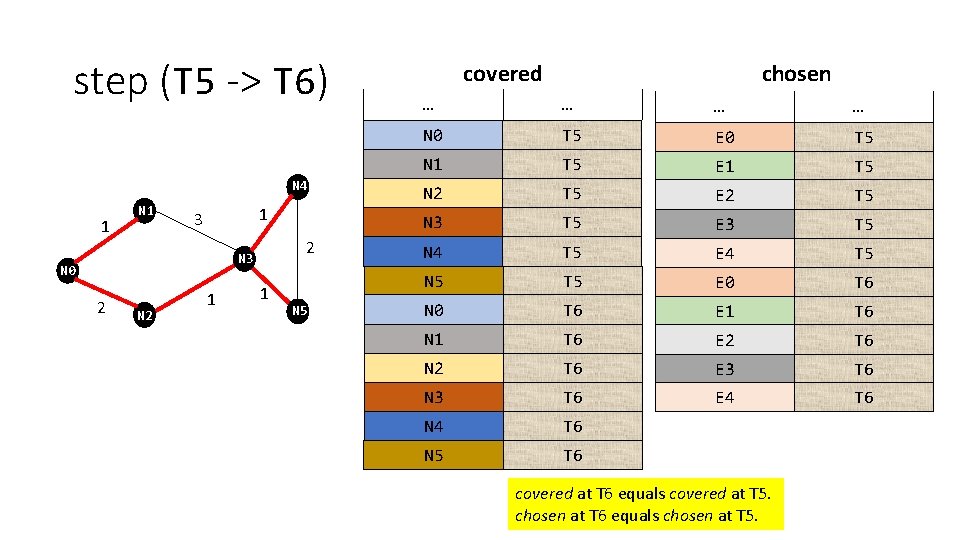
step (T 5 -> T 6) N 4 1 N 1 1 3 2 N 3 N 0 2 N 2 1 1 N 5 covered chosen … … N 0 T 1 T 5 E 0 T 5 N 1 T 5 E 1 T 5 N 2 T 5 E 2 T 5 N 3 T 5 E 3 T 5 N 4 T 5 E 4 T 5 N 5 T 5 E 0 T 6 N 0 T 1 T 6 E 1 T 6 N 1 T 6 E 2 T 6 N 2 T 6 E 3 T 6 N 3 T 6 E 4 T 6 N 5 T 6 covered at T 6 equals covered at T 5. chosen at T 6 equals chosen at T 5.

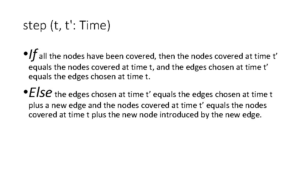
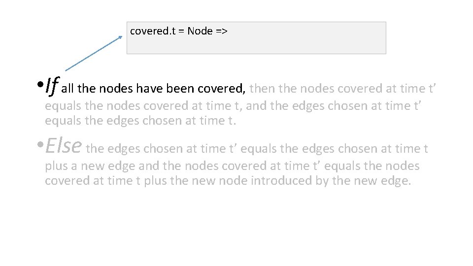
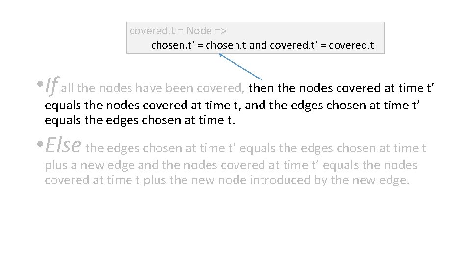
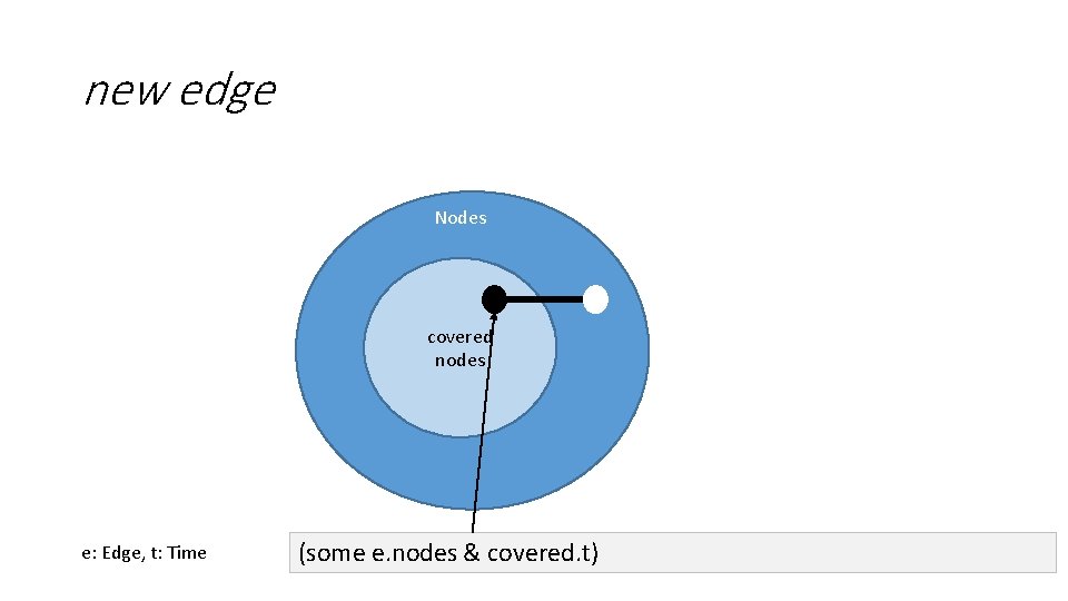
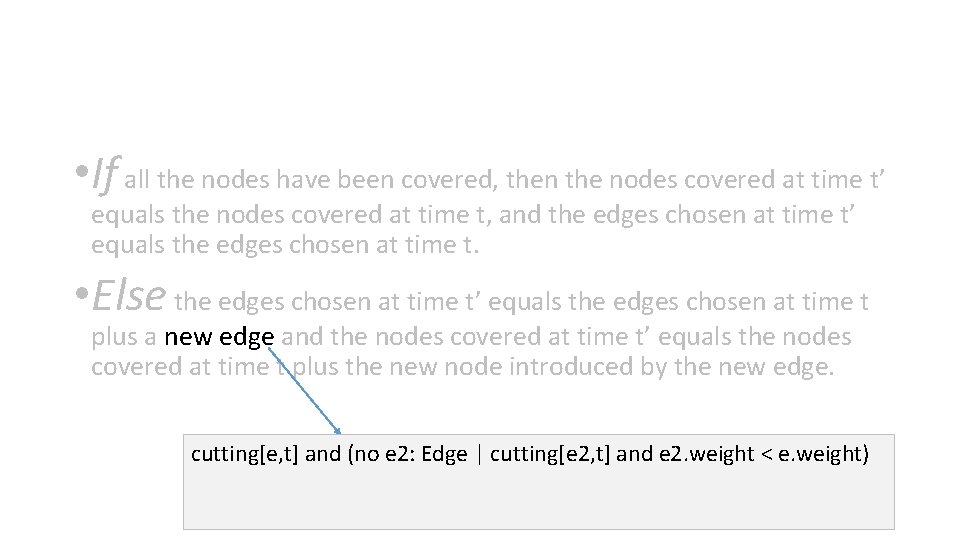
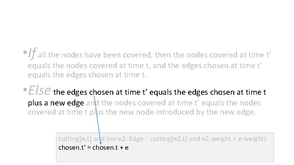
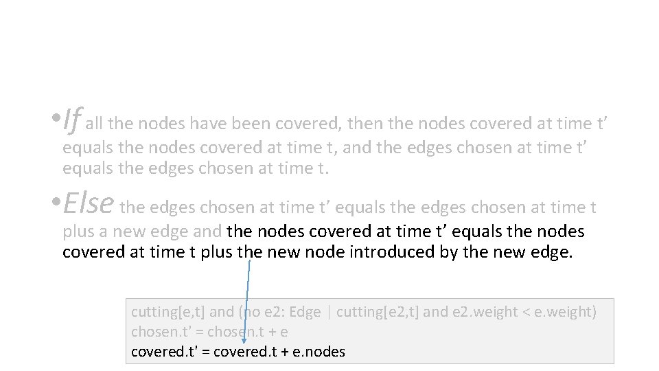
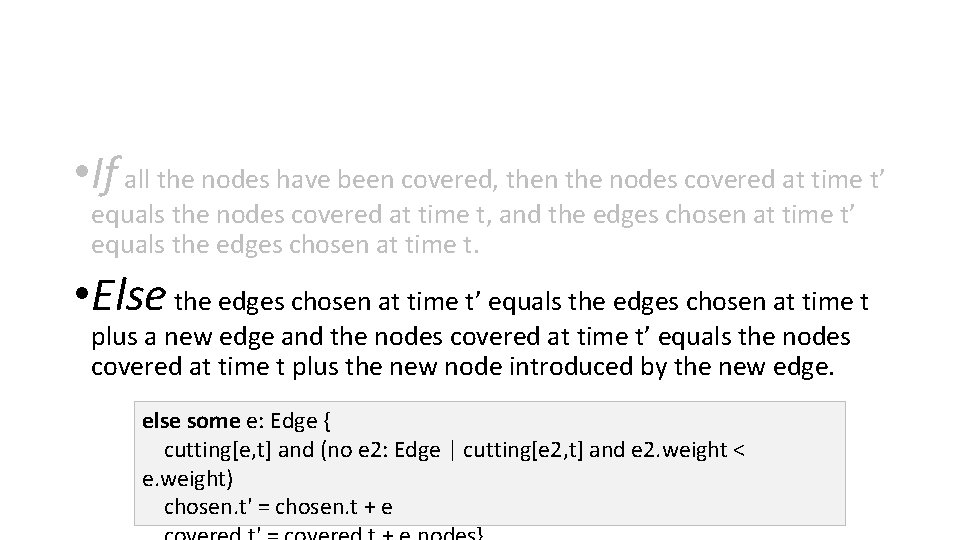
step (t, t': Time) • If all the nodes have been covered, then the nodes covered at time t’ equals the nodes covered at time t, and the edges chosen at time t’ equals the edges chosen at time t. • Else the edges chosen at time t’ equals the edges chosen at time t plus a new edge and the nodes covered at time t’ equals the nodes covered at time t plus the new node introduced by the new edge.

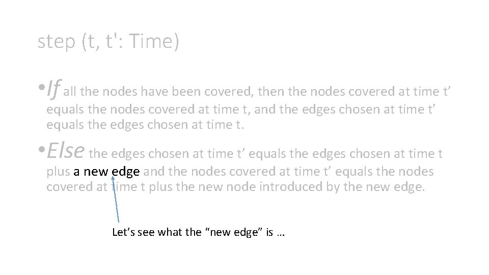
step (t, t': Time) • If all the nodes have been covered, then the nodes covered at time t’ equals the nodes covered at time t, and the edges chosen at time t’ equals the edges chosen at time t. • Else the edges chosen at time t’ equals the edges chosen at time t plus a new edge and the nodes covered at time t’ equals the nodes covered at time t plus the new node introduced by the new edge. Let’s see what the “new edge” is …

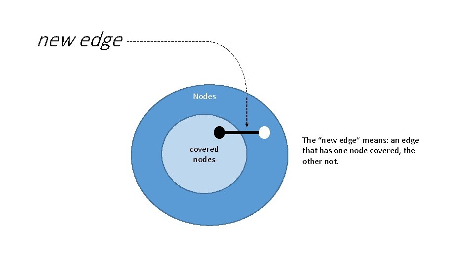
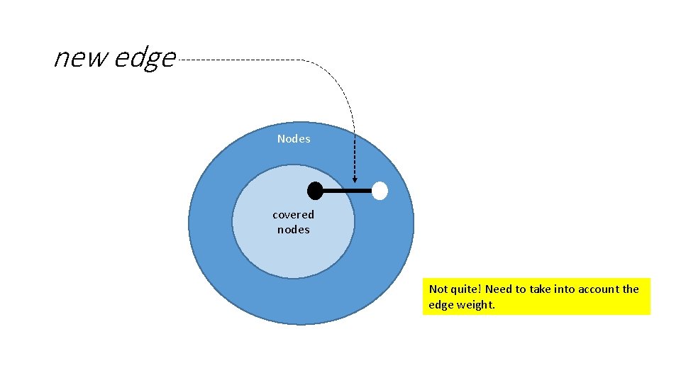
new edge Nodes covered nodes The “new edge” means: an edge that has one node covered, the other not.

new edge Nodes covered nodes Not quite! Need to take into account the edge weight.

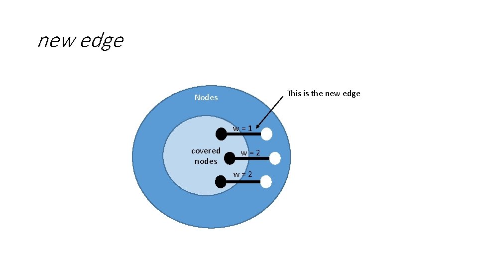
new edge This is the new edge Nodes w=1 covered nodes w=2

covered. t = Node => • If all the nodes have been covered, then the nodes covered at time t’ equals the nodes covered at time t, and the edges chosen at time t’ equals the edges chosen at time t. • Else the edges chosen at time t’ equals the edges chosen at time t plus a new edge and the nodes covered at time t’ equals the nodes covered at time t plus the new node introduced by the new edge.

covered. t = Node => chosen. t' = chosen. t and covered. t' = covered. t • If all the nodes have been covered, then the nodes covered at time t’ equals the nodes covered at time t, and the edges chosen at time t’ equals the edges chosen at time t. • Else the edges chosen at time t’ equals the edges chosen at time t plus a new edge and the nodes covered at time t’ equals the nodes covered at time t plus the new node introduced by the new edge.

new edge Nodes covered nodes e: Edge, t: Time (some e. nodes & covered. t)

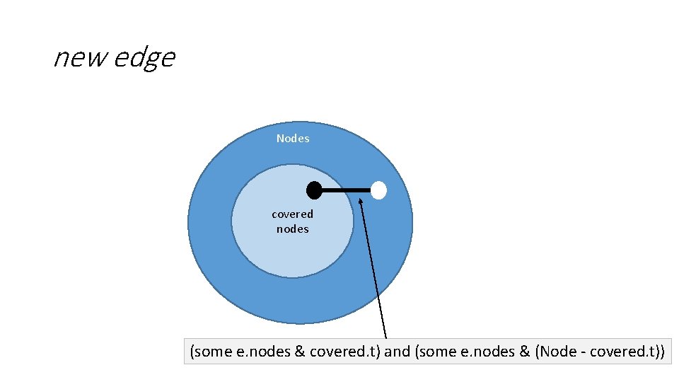
new edge Nodes covered nodes (some e. nodes & covered. t) and (some e. nodes & (Node - covered. t))

new edge Nodes covered nodes (some e. nodes & covered. t) and (some e. nodes & (Node - covered. t))

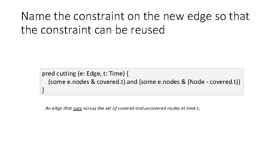
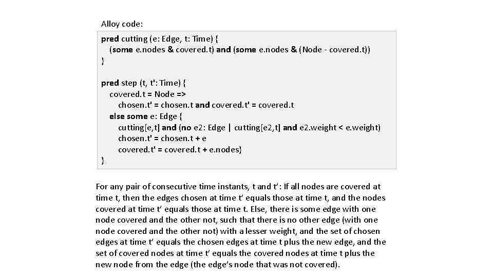
Name the constraint on the new edge so that the constraint can be reused pred cutting (e: Edge, t: Time) { (some e. nodes & covered. t) and (some e. nodes & (Node - covered. t)) } An edge that cuts across the set of covered and uncovered nodes at time t.
![new edge Nodes covered nodes cuttinge t new edge Nodes covered nodes cutting[e, t]](https://slidetodoc.com/presentation_image/58527a0c02aaabfdf71c56ac9909db11/image-73.jpg)
new edge Nodes covered nodes cutting[e, t]
![new edge Nodes W1 covered nodes W2 w2 cuttinge t and no e 2 new edge Nodes W=1 covered nodes W=2 w=2 (cutting[e, t] and (no e 2:](https://slidetodoc.com/presentation_image/58527a0c02aaabfdf71c56ac9909db11/image-74.jpg)
new edge Nodes W=1 covered nodes W=2 w=2 (cutting[e, t] and (no e 2: Edge | cutting[e 2, t] and e 2. weight < e. weight)

• If all the nodes have been covered, then the nodes covered at time t’ equals the nodes covered at time t, and the edges chosen at time t’ equals the edges chosen at time t. • Else the edges chosen at time t’ equals the edges chosen at time t plus a new edge and the nodes covered at time t’ equals the nodes covered at time t plus the new node introduced by the new edge. cutting[e, t] and (no e 2: Edge | cutting[e 2, t] and e 2. weight < e. weight)

• If all the nodes have been covered, then the nodes covered at time t’ equals the nodes covered at time t, and the edges chosen at time t’ equals the edges chosen at time t. • Else the edges chosen at time t’ equals the edges chosen at time t plus a new edge and the nodes covered at time t’ equals the nodes covered at time t plus the new node introduced by the new edge. cutting[e, t] and (no e 2: Edge | cutting[e 2, t] and e 2. weight < e. weight) chosen. t' = chosen. t + e

• If all the nodes have been covered, then the nodes covered at time t’ equals the nodes covered at time t, and the edges chosen at time t’ equals the edges chosen at time t. • Else the edges chosen at time t’ equals the edges chosen at time t plus a new edge and the nodes covered at time t’ equals the nodes covered at time t plus the new node introduced by the new edge. cutting[e, t] and (no e 2: Edge | cutting[e 2, t] and e 2. weight < e. weight) chosen. t' = chosen. t + e covered. t' = covered. t + e. nodes

• If all the nodes have been covered, then the nodes covered at time t’ equals the nodes covered at time t, and the edges chosen at time t’ equals the edges chosen at time t. • Else the edges chosen at time t’ equals the edges chosen at time t plus a new edge and the nodes covered at time t’ equals the nodes covered at time t plus the new node introduced by the new edge. else some e: Edge { cutting[e, t] and (no e 2: Edge | cutting[e 2, t] and e 2. weight < e. weight) chosen. t' = chosen. t + e

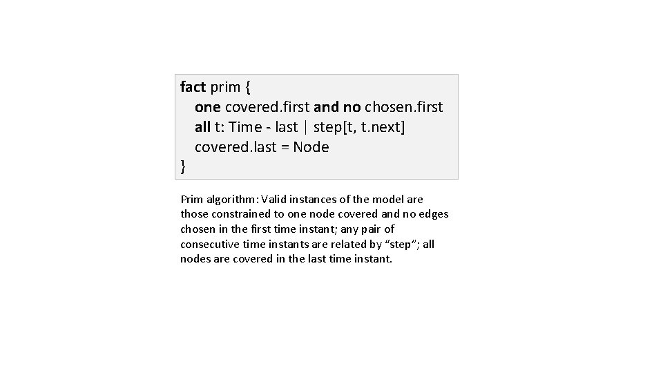
Alloy code: pred cutting (e: Edge, t: Time) { (some e. nodes & covered. t) and (some e. nodes & (Node - covered. t)) } pred step (t, t': Time) { covered. t = Node => chosen. t' = chosen. t and covered. t' = covered. t else some e: Edge { cutting[e, t] and (no e 2: Edge | cutting[e 2, t] and e 2. weight < e. weight) chosen. t' = chosen. t + e covered. t' = covered. t + e. nodes} } For any pair of consecutive time instants, t and t’: If all nodes are covered at time t, then the edges chosen at time t’ equals those at time t, and the nodes covered at time t’ equals those at time t. Else, there is some edge with one node covered and the other not, such that there is no other edge (with one node covered and the other not) with a lesser weight, and the set of chosen edges at time t’ equals the chosen edges at time t plus the new edge, and the set of covered nodes at time t’ equals the covered nodes at time t plus the new node from the edge (the edge’s node that was not covered).

fact prim { one covered. first and no chosen. first all t: Time - last | step[t, t. next] covered. last = Node } Prim algorithm: Valid instances of the model are those constrained to one node covered and no edges chosen in the first time instant; any pair of consecutive time instants are related by “step”; all nodes are covered in the last time instant.
![open utilorderingTime sig Time sig Node covered set Time sig Edge weight Int open util/ordering[Time] sig Time {} sig Node {covered: set Time} sig Edge {weight: Int,](https://slidetodoc.com/presentation_image/58527a0c02aaabfdf71c56ac9909db11/image-81.jpg)
open util/ordering[Time] sig Time {} sig Node {covered: set Time} sig Edge {weight: Int, nodes: set Node, chosen: set Time} { weight >= 0 and #nodes = 2 } pred cutting (e: Edge, t: Time) { (some e. nodes & covered. t) and (some e. nodes & (Node - covered. t)) } pred step (t, t': Time) { covered. t = Node => chosen. t' = chosen. t and covered. t' = covered. t else some e: Edge { cutting[e, t] and (no e 2: Edge | cutting[e 2, t] and e 2. weight < e. weight) chosen. t' = chosen. t + e covered. t' = covered. t + e. nodes} } fact prim { one covered. first and no chosen. first all t: Time - last | step[t, t. next] covered. last = Node } We have used the Alloy language to declaratively model the Prim algorithm!

For comparison, let’s see a procedural description (C code) of the Prim algorithm …
![primgraph g int start int i edgenode p bool intreeMAXV1 int distanceMAXV1 int prim(graph *g, int start) { int i; edgenode *p; bool intree[MAXV+1]; int distance[MAXV+1] int](https://slidetodoc.com/presentation_image/58527a0c02aaabfdf71c56ac9909db11/image-83.jpg)
prim(graph *g, int start) { int i; edgenode *p; bool intree[MAXV+1]; int distance[MAXV+1] int v; int weight; int dist; for (i=1; i<=g->nvertices; i++) { intree[i] = FALSE; distance[i] = MAXINT; parent[i] = -1; } distance[start] = 0; v = start; while (intree[v] == FALSE) { intree[v] = TRUE; p = g->edges[v]; while (p!= NULL) { w = p->y; weight = p->weight; if ((distance[w] > weight) && (intree[w] == FALSE)) { distance[w] = weight; parent[w] = v; } p = p->next; } This code comes from the book The Algorithm Design Manual by Steven S. Skiena, page 194 -195. } } v = 1; dist = MAXINT; for (i=1; i<=g->nvertices; i++) if ((intree[i] == FALSE) && (dist > distance[i])) { dist = distance[i]; v = 1; } Roger’s opinion: Wow, this is so different from the declarative model. The declarative model focuses on the key abstractions/concepts (nodes and edges), and how they are selected based on edge weight. Conversely, this procedural description is bogged down in irrelevant minutia.

The model is finished! • We declaratively modeled the structural components (Node and Edge) and relations (covered, weight, nodes, and chosen). • Then we defined the constraints that must hold among the structural components and relations. • Now let’s test the model. Let’s see if: 1. The set of nodes and edges that are valid per the model’s constraints form a “spanning tree. ” 2. The set of nodes and edges form a “minimum spanning tree. ”

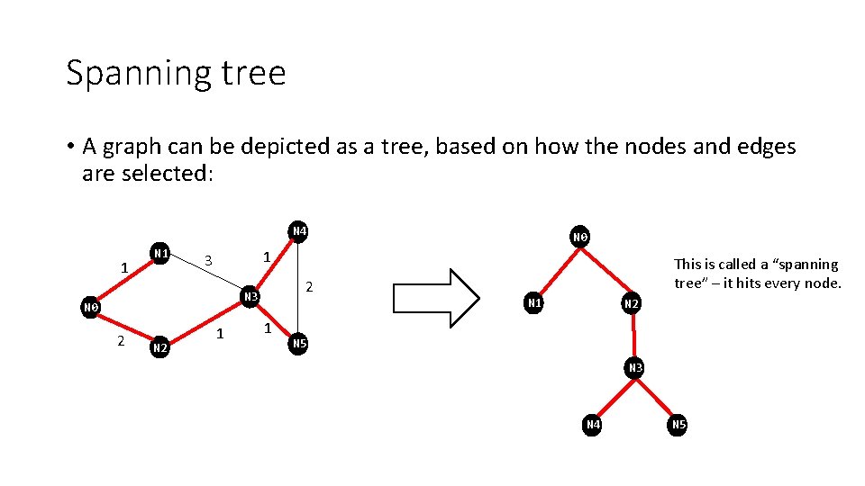
Spanning tree • A graph can be depicted as a tree, based on how the nodes and edges are selected: N 4 1 N 1 1 3 2 N 3 N 0 2 N 0 1 1 This is called a “spanning tree” – it hits every node. N 1 N 2 N 5 N 3 N 4 N 5

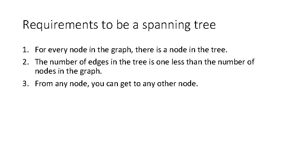
Requirements to be a spanning tree 1. For every node in the graph, there is a node in the tree. 2. The number of edges in the tree is one less than the number of nodes in the graph. 3. From any node, you can get to any other node.

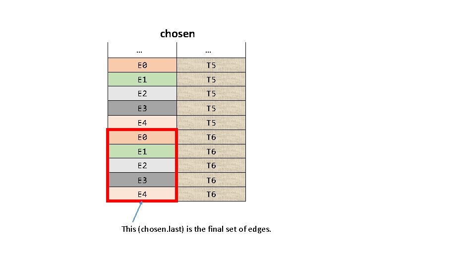
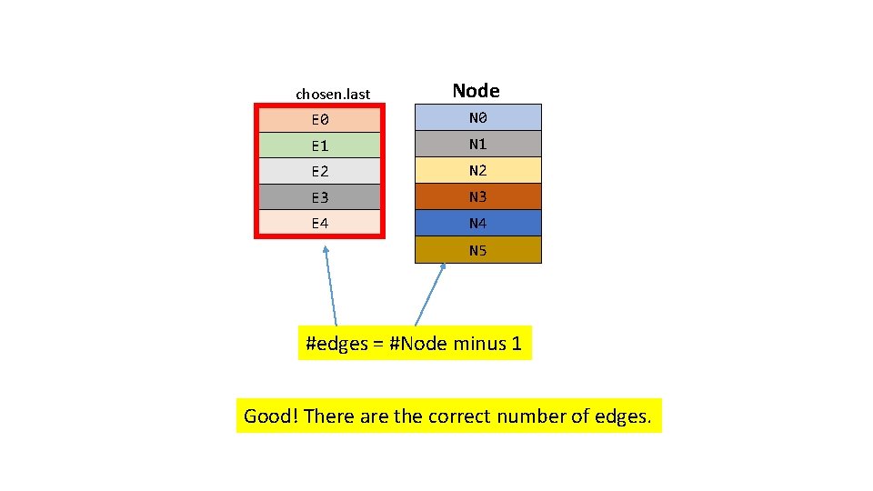
chosen … … E 0 T 5 E 1 T 5 E 2 T 5 E 3 T 5 E 4 T 5 E 0 T 6 E 1 T 6 E 2 T 6 E 3 T 6 E 4 T 6 This (chosen. last) is the final set of edges.

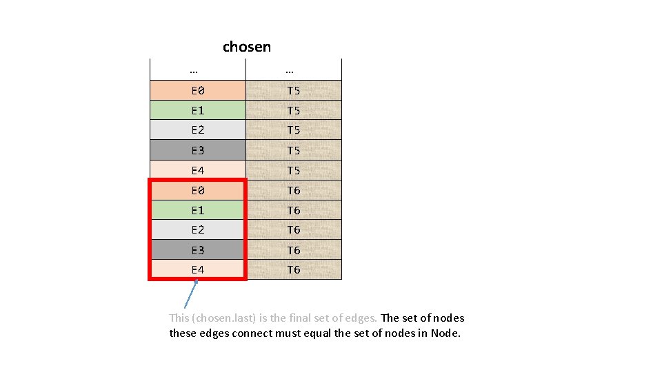
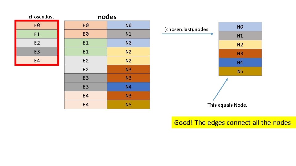
chosen … … E 0 T 5 E 1 T 5 E 2 T 5 E 3 T 5 E 4 T 5 E 0 T 6 E 1 T 6 E 2 T 6 E 3 T 6 E 4 T 6 This (chosen. last) is the final set of edges. The set of nodes these edges connect must equal the set of nodes in Node.

nodes chosen. last E 0 N 0 E 1 E 0 N 1 E 2 E 1 N 0 N 2 E 3 E 1 N 2 N 3 E 4 E 2 N 3 N 5 E 3 N 3 E 3 N 4 E 4 N 3 E 4 N 5 (chosen. last). nodes N 0 N 1 This equals Node. Good! The edges connect all the nodes.

chosen. last Node E 0 N 0 E 1 N 1 E 2 N 2 E 3 N 3 E 4 N 5 #edges = #Node minus 1 Good! There are the correct number of edges.

Requirements to be a spanning tree 1. For every node in the graph, there is a node in the tree. 2. The number of edges in the tree is one less than the number of nodes in the graph. 3. From any node, you can get to any other node. Done!

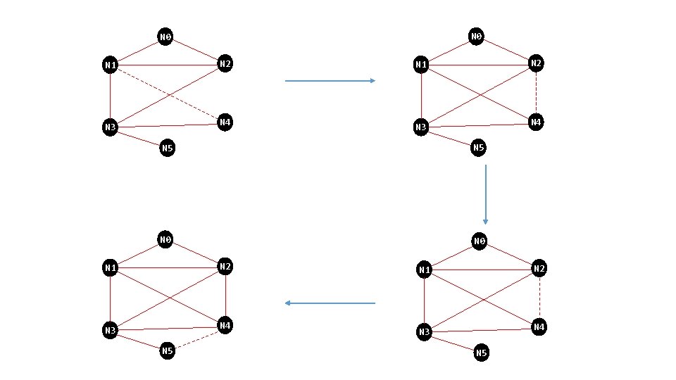
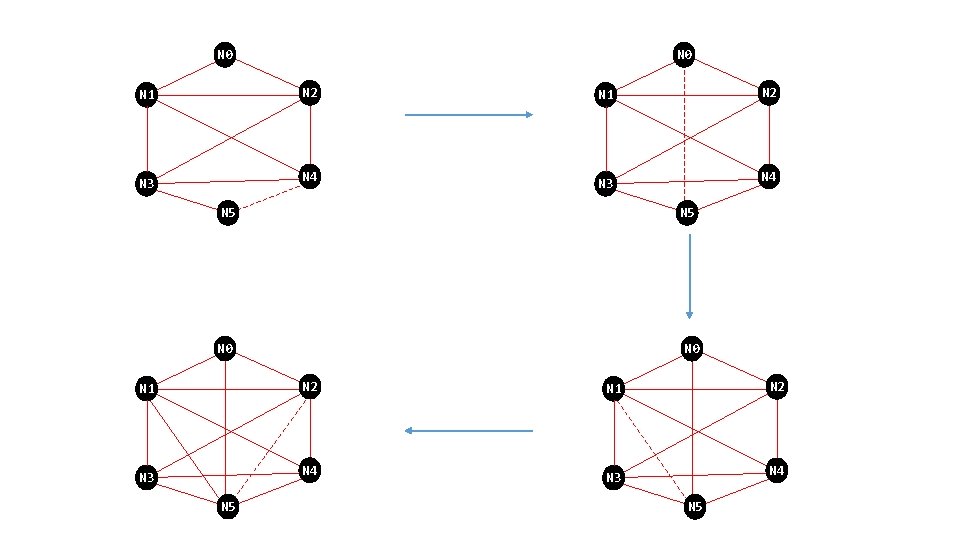
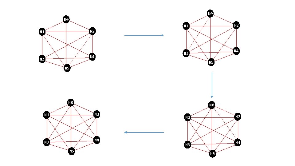
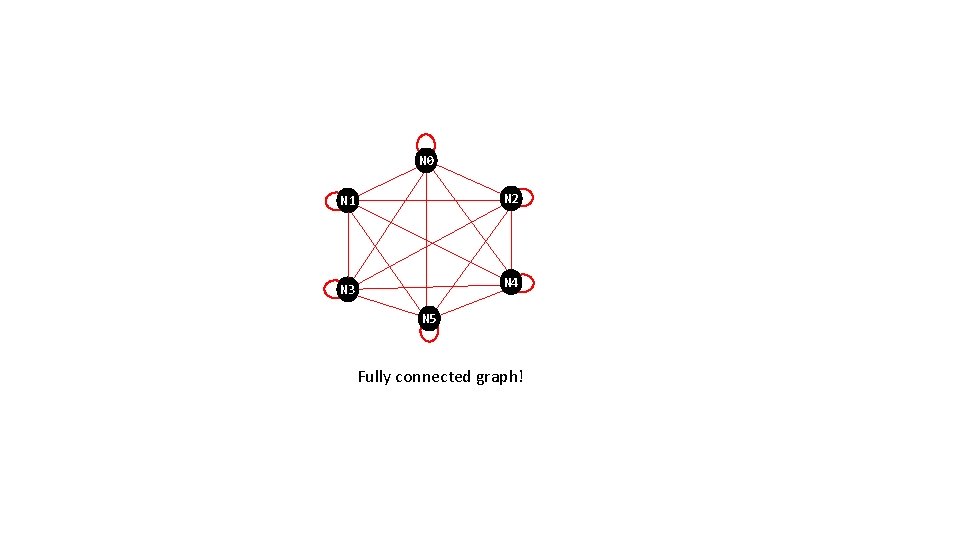
Requirements to be a spanning tree 1. For every node in the graph, there is a node in the tree. 2. The number of edges in the tree is one less than the number of nodes in the graph. 3. From any node, you can get to any other node. Let’s work on this. But first, let’s see what a “fully connected” graph is.

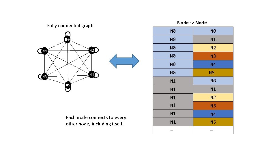
Fully connected graph N 0 N 2 N 1 N 4 N 3 N 5 Each node connects to every other node, including itself. Node -> Node N 0 N 0 N 1 N 0 N 2 N 0 N 3 N 0 N 4 N 0 N 5 N 1 N 0 N 1 N 1 N 2 N 1 N 4 N 5 … N 1 … N 3

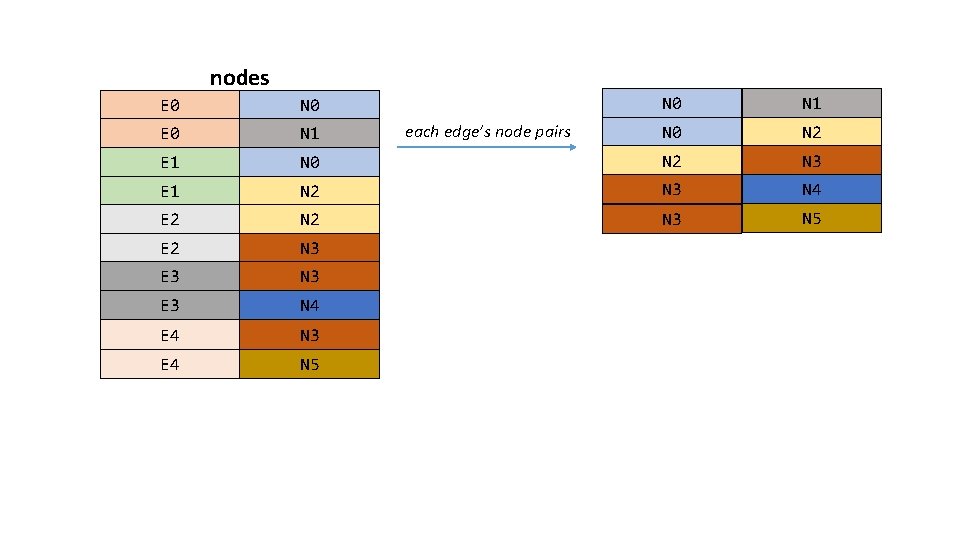
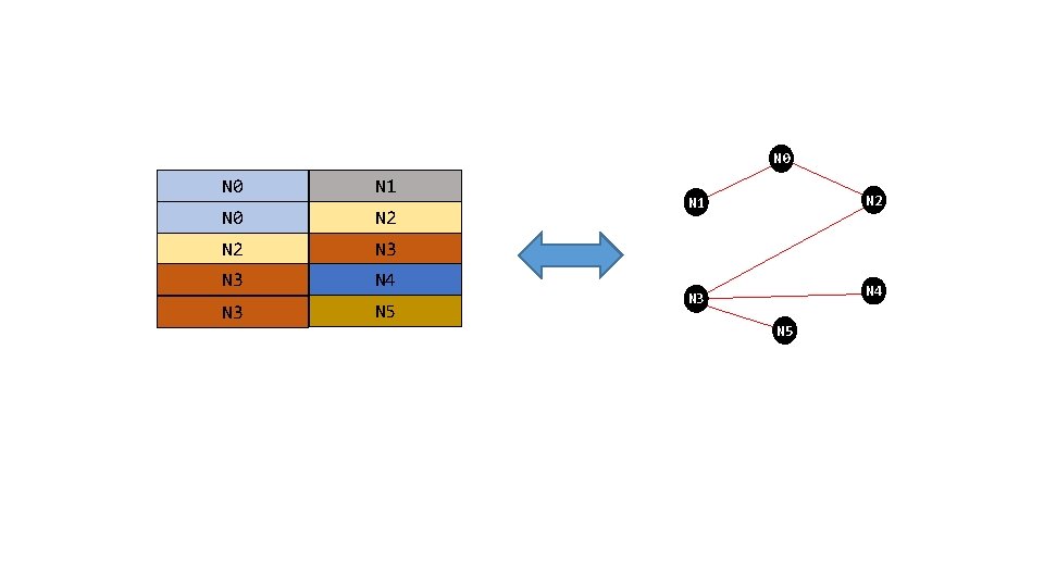
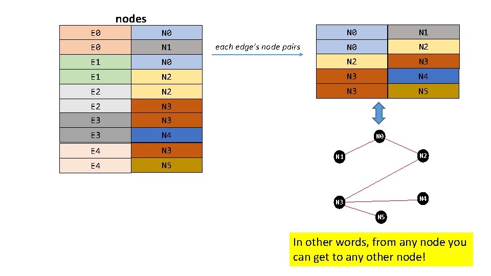
nodes N 0 N 1 N 0 N 2 N 3 E 1 N 2 N 3 N 4 E 2 N 3 N 5 E 2 N 3 E 3 N 4 E 4 N 3 E 4 N 5 E 0 N 0 E 0 N 1 E 1 each edge’s node pairs

N 0 N 1 N 0 N 2 N 3 N 4 N 3 N 5 N 2 N 1 N 4 N 3 N 5

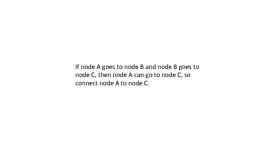
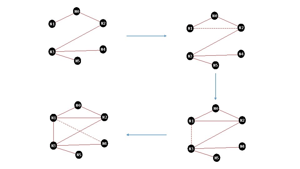
If node A goes to node B and node B goes to node C, then node A can go to node C, so connect node A to node C.

N 0 N 2 N 1 N 4 N 3 N 5 N 0 N 2 N 1 N 4 N 3 N 5

N 0 N 2 N 1 N 4 N 3 N 5

N 0 N 2 N 1 N 4 N 3 N 5 N 0 N 2 N 4 N 3 N 5 N 1 N 2 N 1 N 4 N 3 N 5

N 0 N 2 N 1 N 4 N 3 N 5

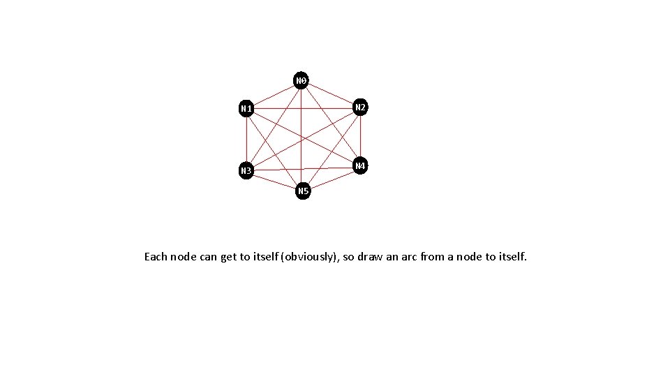
N 0 N 2 N 1 N 4 N 3 N 5 Each node can get to itself (obviously), so draw an arc from a node to itself.

N 0 N 2 N 1 N 4 N 3 N 5 Fully connected graph!

nodes N 0 N 1 N 0 N 2 N 3 E 1 N 2 N 3 N 4 E 2 N 3 N 5 E 2 N 3 E 3 N 4 E 4 N 3 E 4 N 5 E 0 N 0 E 0 N 1 E 1 each edge’s node pairs N 0 N 2 N 1 N 4 N 3 N 5 In other words, from any node you can get to any other node!

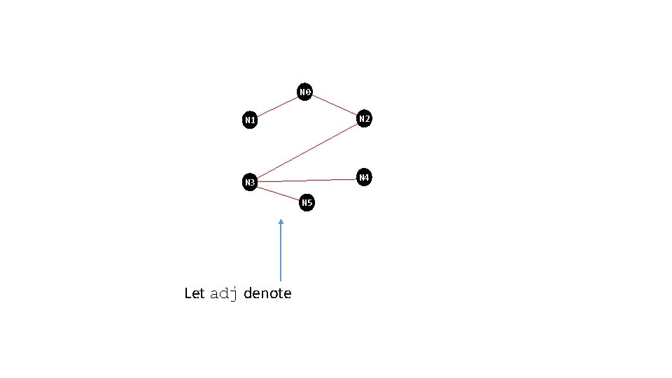
N 0 N 2 N 1 N 4 N 3 N 5 Let adj denote

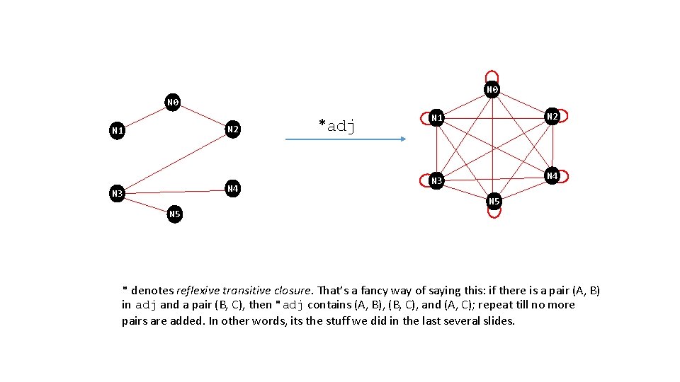
N 0 N 2 N 1 N 4 N 3 *adj N 2 N 1 N 4 N 3 N 5 * denotes reflexive transitive closure. That’s a fancy way of saying this: if there is a pair (A, B) in adj and a pair (B, C), then *adj contains (A, B), (B, C), and (A, C); repeat till no more pairs are added. In other words, its the stuff we did in the last several slides.

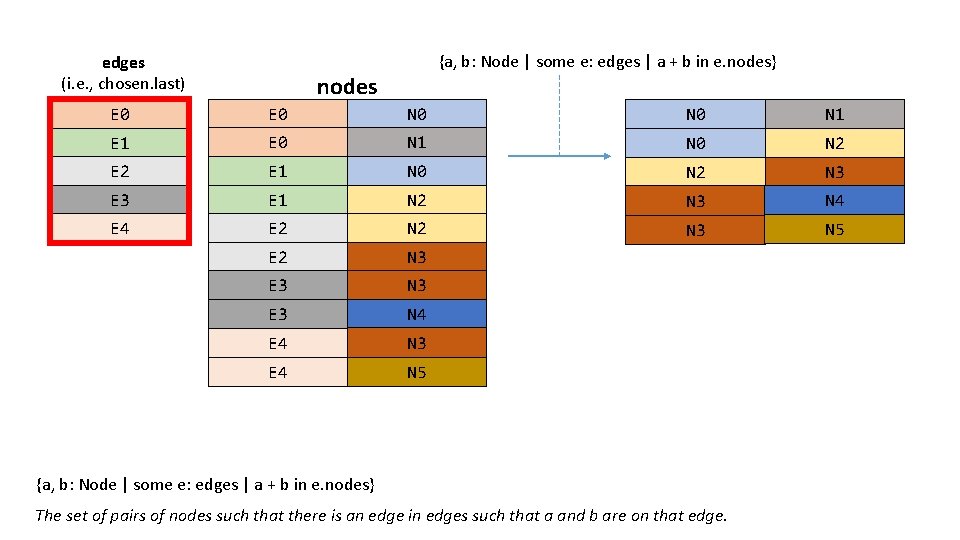
edges (i. e. , chosen. last) {a, b: Node | some e: edges | a + b in e. nodes} nodes E 0 N 0 N 1 E 0 N 1 N 0 N 2 E 1 N 0 N 2 N 3 E 1 N 2 N 3 N 4 E 2 N 3 N 5 E 2 N 3 E 3 N 4 E 4 N 3 E 4 N 5 {a, b: Node | some e: edges | a + b in e. nodes} The set of pairs of nodes such that there is an edge in edges such that a and b are on that edge.

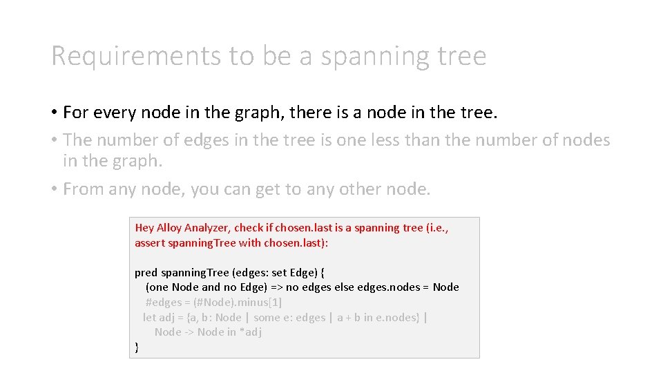
Requirements to be a spanning tree • For every node in the graph, there is a node in the tree. • The number of edges in the tree is one less than the number of nodes in the graph. • From any node, you can get to any other node. Hey Alloy Analyzer, check if chosen. last is a spanning tree (i. e. , assert spanning. Tree with chosen. last): pred spanning. Tree (edges: set Edge) { (one Node and no Edge) => no edges else edges. nodes = Node #edges = (#Node). minus[1] let adj = {a, b: Node | some e: edges | a + b in e. nodes} | Node -> Node in *adj }

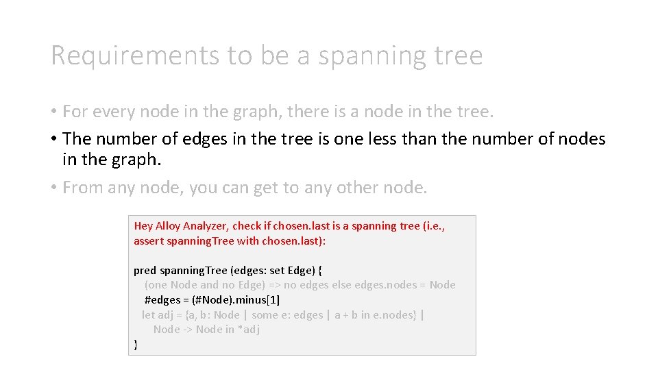
Requirements to be a spanning tree • For every node in the graph, there is a node in the tree. • The number of edges in the tree is one less than the number of nodes in the graph. • From any node, you can get to any other node. Hey Alloy Analyzer, check if chosen. last is a spanning tree (i. e. , assert spanning. Tree with chosen. last): pred spanning. Tree (edges: set Edge) { (one Node and no Edge) => no edges else edges. nodes = Node #edges = (#Node). minus[1] let adj = {a, b: Node | some e: edges | a + b in e. nodes} | Node -> Node in *adj }

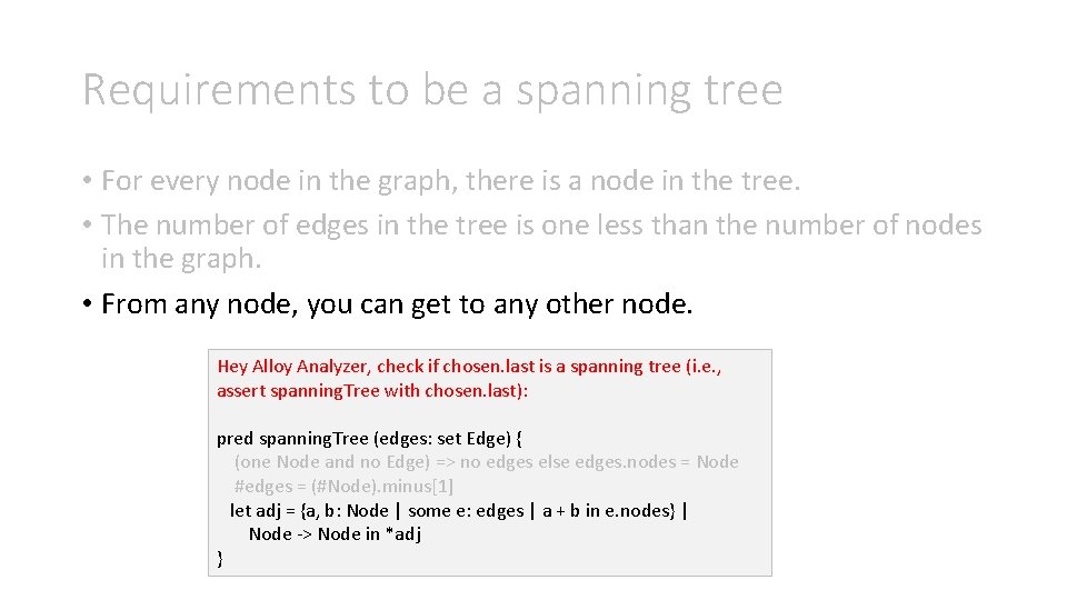
Requirements to be a spanning tree • For every node in the graph, there is a node in the tree. • The number of edges in the tree is one less than the number of nodes in the graph. • From any node, you can get to any other node. Hey Alloy Analyzer, check if chosen. last is a spanning tree (i. e. , assert spanning. Tree with chosen. last): pred spanning. Tree (edges: set Edge) { (one Node and no Edge) => no edges else edges. nodes = Node #edges = (#Node). minus[1] let adj = {a, b: Node | some e: edges | a + b in e. nodes} | Node -> Node in *adj }
![correct check spanning Tree chosen last for 5 but 10 Edge 5 correct: check { spanning. Tree [chosen. last] } for 5 but 10 Edge, 5](https://slidetodoc.com/presentation_image/58527a0c02aaabfdf71c56ac9909db11/image-110.jpg)
correct: check { spanning. Tree [chosen. last] } for 5 but 10 Edge, 5 Int Alloy Analyzer

We checked our model to see if its instances are spanning trees. The Alloy Analyzer found no counterexamples!

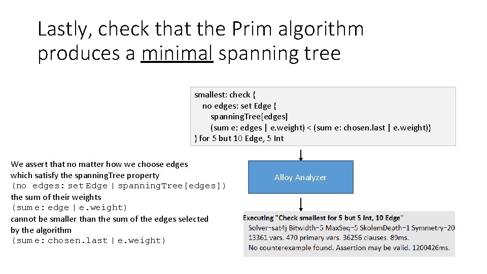
Lastly, check that the Prim algorithm produces a minimal spanning tree smallest: check { no edges: set Edge { spanning. Tree[edges] (sum e: edges | e. weight) < (sum e: chosen. last | e. weight)} } for 5 but 10 Edge, 5 Int We assert that no matter how we choose edges which satisfy the spanning. Tree property (no edges: set Edge | spanning. Tree[edges]) the sum of their weights (sum e: edge | e. weight) cannot be smaller than the sum of the edges selected by the algorithm (sum e: chosen. last | e. weight) Alloy Analyzer

Be sure that you’ve selected “Prevent overflows: Yes”

We checked our model to see if its instances are minimal spanning trees. The Alloy Analyzer found no counterexamples!

Done!

Well, one more thing. An interesting tidbit about Alloy …

Alloy is an idiomless language • Alloy doesn’t have a fixed idiom for models, so you are free to use whatever idiom works best for the model at hand. • For example, the event idiom is well-suited to modeling “hotel operations, ” which involve events such as check-in, checkout, and room entry.