Using a Particle Dispersion Model to Assess Ventilation




- Slides: 22

Using a Particle Dispersion Model to Assess Ventilation Adjective Ratings in Colorado Joseph J. Charney 1, Michael T. Kiefer 2, Shiyuan Zhong 2, Warren E. Heilman 1, Xindi Bian 1, and Tim Mathewson 3 1 USDA Forest Service, Northern Research Station, Lansing, MI 2 Michigan State University, Department of Geography, Environment and Spatial Sciences, East Lansing, MI 3 US Department of the Interior, Bureau of Land Management, Lakewood, CO

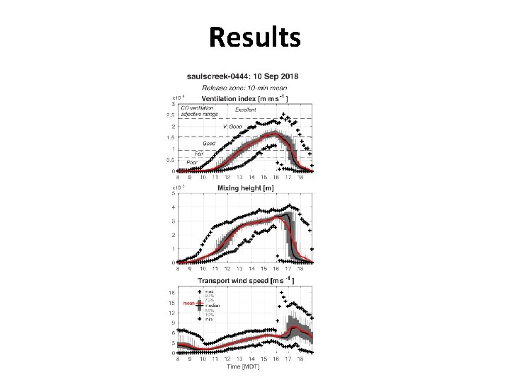
Background • Ventilation index (VI) describes potential for pollutant to ventilate away from source – VAR used as diagnostic tool by fire managers to assess potential for smoke to disperse from a prescribed fire • Smoke dispersion in complex terrain subject of ongoing research • Utility of VI for indicating dispersion potential remains largely undocumented, especially in complex terrain

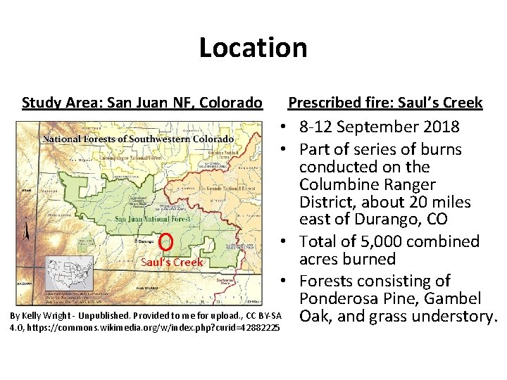
Location Study Area: San Juan NF, Colorado Prescribed fire: Saul’s Creek • 8 -12 September 2018 • Part of series of burns conducted on the Columbine Ranger District, about 20 miles east of Durango, CO • Total of 5, 000 combined acres burned Saul’s Creek • Forests consisting of Ponderosa Pine, Gambel By Kelly Wright - Unpublished. Provided to me for upload. , CC BY-SA Oak, and grass understory. 4. 0, https: //commons. wikimedia. org/w/index. php? curid=42882225

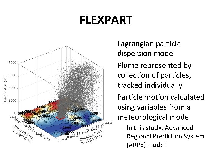
FLEXPART • Lagrangian particle dispersion model • Plume represented by collection of particles, tracked individually • Particle motion calculated using variables from a meteorological model – In this study: Advanced Regional Prediction System (ARPS) model

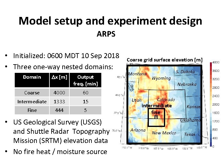
Model setup and experiment design ARPS • Initialized: 0600 MDT 10 Sep 2018 • Three one-way nested domains: Domain Dx [m] Output freq. [min] Coarse 4000 60 Intermediate 1333 15 Fine 444 5 • US Geological Survey (USGS) and Shuttle Radar Topography Mission (SRTM) elevation data • No fire heat / moisture source Coarse grid surface elevation [m] Montana S. Dakota Wyoming Nebraska Utah Colorado intermediate fine Kansas Oklahoma Arizona New Mexico Texas

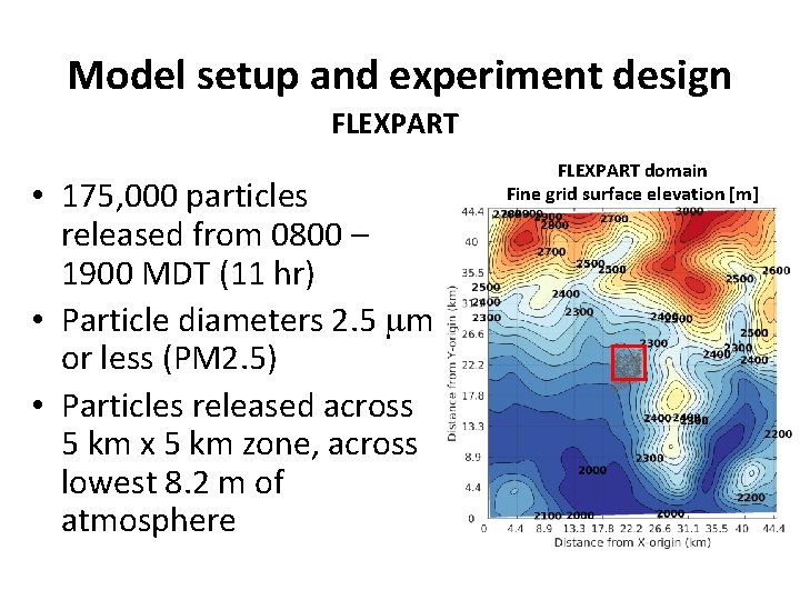
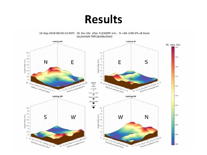
Model setup and experiment design FLEXPART • 175, 000 particles released from 0800 – 1900 MDT (11 hr) • Particle diameters 2. 5 mm or less (PM 2. 5) • Particles released across 5 km x 5 km zone, across lowest 8. 2 m of atmosphere FLEXPART domain Fine grid surface elevation [m]

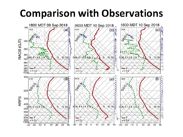
Comparison with Observations

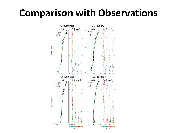
Comparison with Observations

Results

Results

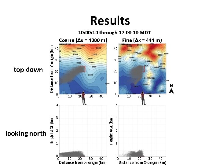
Results 40 40 30 30 20 20 10 10 0 0 10 20 30 0 0 40 4 4 3 3 Height AGL (km) looking north Height AGL (km) top down Distance from Y-origin (km) 10: 00: 10 through 17: 00: 10 MDT Coarse (Dx = 4000 m) Fine (Dx = 444 m) 2 1 0 0 10 20 30 40 Distance from X-origin (km) 10 20 30 40 2 1 0 0 Distance from X-origin (km)

Results

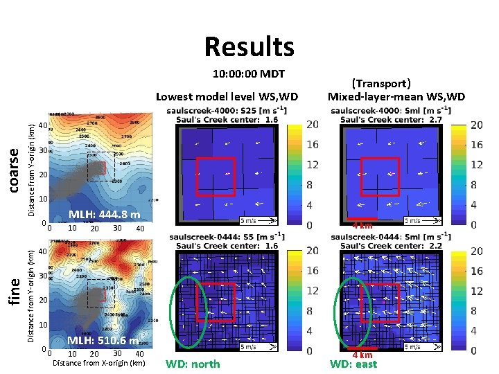
Results 10: 00 MDT Distance from Y-origin (km) coarse Lowest model level WS, WD 40 30 20 10 MLH: 444. 8 m Distance from Y-origin (km) 0 fine (Transport) Mixed-layer-mean WS, WD 0 10 20 30 4 km 40 40 30 20 10 0 MLH: 510. 6 m 0 30 10 40 20 Distance from X-origin (km) WD: north 4 km WD: east

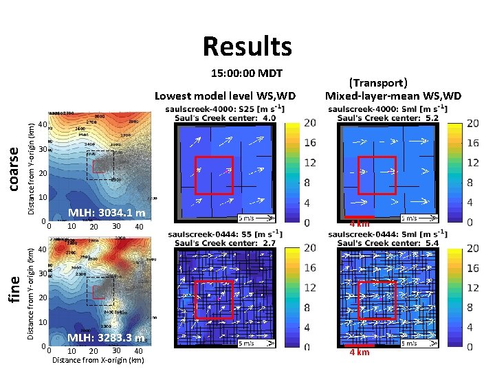
Results 15: 00 MDT Distance from Y-origin (km) coarse Lowest model level WS, WD 40 30 20 10 MLH: 3034. 1 m Distance from Y-origin (km) 0 fine (Transport) Mixed-layer-mean WS, WD 0 10 20 30 40 4 km 40 30 20 10 0 MLH: 3283. 3 m 0 30 10 40 20 Distance from X-origin (km) 4 km

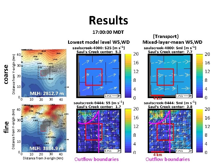
Results 17: 00 MDT Distance from Y-origin (km) coarse Lowest model level WS, WD 40 30 20 10 MLH: 2812. 7 m Distance from Y-origin (km) 0 fine (Transport) Mixed-layer-mean WS, WD 0 10 20 30 4 km 40 40 30 20 10 0 MLH: 3884. 9 m 0 30 10 40 20 Distance from X-origin (km) Outflow boundaries 4 km Outflow boundaries

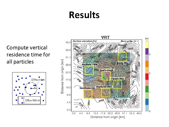
Results Analysis procedure 1. Compute residence time for all particles 2. Define analysis zones to compare particle dispersion in different areas of domain

Results Compute vertical residence time for all particles

Results

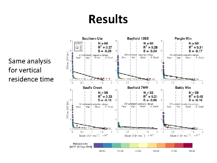
Results Analysis procedure 3. Compute ensembleaverage residence time and compare to time- and zoneaveraged VI • Bin all particles released in each zone, during each 10 -minute time block.

Thunderstorm Outflow

Results Same analysis for vertical residence time

Discussion Points • Clear differences in relationship better VAR and dispersion at different elevations – Could/should these differences be quantified and applied to smoke management decisions? • Clear effect of meteorology resolution on the dispersion prediction – Comparisons with observations could/should yield recommended grid spacing for smoke dispersion prediction • How can meteorological data at the required resolution be made available in real time?