Use of moment generating functions 1 Using the

Use of moment generating functions 1. Using the moment generating functions of X, Y, Z, …determine the moment generating function of W = h(X, Y, Z, …). 2. Identify the distribution of W from its moment generating function This procedure works well for sums, linear combinations etc.

Therorem Let X and Y denote a independent random variables each having a gamma distribution with parameters (l, a 1) and (l, a 2). Then W = X + Y has a gamma distribution with parameters (l, a 1 + a 2). Proof:

Recognizing that this is the moment generating function of the gamma distribution with parameters (l, a 1 + a 2) we conclude that W = X + Y has a gamma distribution with parameters (l, a 1 + a 2).

Therorem (extension to n RV’s) Let x 1, x 2, … , xn denote n independent random variables each having a gamma distribution with parameters (l, ai), i = 1, 2, …, n. Then W = x 1 + x 2 + … + xn has a gamma distribution with parameters (l, a 1 + a 2 +… + an). Proof:

Therefore Recognizing that this is the moment generating function of the gamma distribution with parameters (l, a 1 + a 2 +…+ an) we conclude that W = x 1 + x 2 + … + xn has a gamma distribution with parameters (l, a 1 + a 2 +…+ an).

Therorem Suppose that x is a random variable having a gamma distribution with parameters (l, a). Then W = ax has a gamma distribution with parameters (l/a, a). Proof:

Special Cases 1. Let X and Y be independent random variables having a c 2 distribution with n 1 and n 2 degrees of freedom respectively then X + Y has a c 2 distribution with degrees of freedom n 1 + n 2. 2. Let x 1, x 2, …, xn, be independent random variables having a c 2 distribution with n 1 , n 2 , …, nn degrees of freedom respectively then x 1+ x 2 +…+ xn has a c 2 distribution with degrees of freedom n 1 +…+ nn. Both of these properties follow from the fact that a c 2 random variable with n degrees of freedom is a G random variable with l = ½ and a = n/2.

Recall If z has a Standard Normal distribution then z 2 has a c 2 distribution with 1 degree of freedom. Thus if z 1, z 2, …, zn are independent random variables each having Standard Normal distribution then has a c 2 distribution with n degrees of freedom.

Therorem Suppose that U 1 and U 2 are independent random variables and that U = U 1 + U 2 Suppose that U 1 and U have a c 2 distribution with degrees of freedom n 1 andn respectively. (n 1 < n) Then U 2 has a c 2 distribution with degrees of freedom n 2 =n -n 1 Proof:

Q. E. D.

Distribution of the sample variance

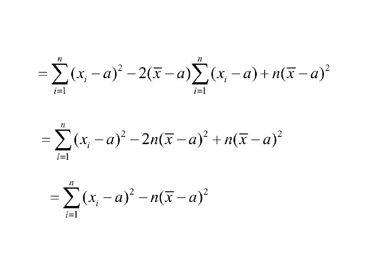
Properties of the sample variance Proof:

Special Cases 1. Setting a = 0. Computing formula

2. Setting a = m.

Distribution of the sample variance Let x 1, x 2, …, xn denote a sample from the normal distribution with mean m and variance s 2. Let Then has a c 2 distribution with n degrees of freedom.

Note: or U = U 2 + U 1 has a c 2 distribution with n degrees of freedom.

We also know that has normal distribution with mean m and variance s 2/n Thus has a Standard Normal distribution and has a c 2 distribution with 1 degree of freedom.

If we can show that U 1 and U 2 are independent then has a c 2 distribution with n - 1 degrees of freedom. The final task would be to show that are independent

Summary Let x 1, x 2, …, xn denote a sample from the normal distribution with mean m and variance s 2. 1. than has normal distribution with mean m and variance s 2/n 2. has a c 2 distribution with n = n - 1 degrees of freedom.

The Transformation Method Theorem Let X denote a random variable with probability density function f(x) and U = h(X). Assume that h(x) is either strictly increasing (or decreasing) then the probability density of U is:

Proof Use the distribution function method. Step 1 Find the distribution function, G(u) Step 2 Differentiate G (u ) to find the probability density function g(u)

hence

or

Example Suppose that X has a Normal distribution with mean m and variance s 2. Find the distribution of U = h(x) = e. X. Solution:

hence This distribution is called the log-normal distribution

log-normal distribution

The Transfomation Method (many variables) Theorem Let x 1, x 2, …, xn denote random variables with joint probability density function f(x 1, x 2, …, xn ) Let u 1 = h 1(x 1, x 2, …, xn). u 2 = h 2(x 1, x 2, …, xn). un = hn(x 1, x 2, …, xn). define an invertible transformation from the x’s to the u’s

Then the joint probability density function of u 1, u 2, …, un is given by: where Jacobian of the transformation

Example Suppose that x 1, x 2 are independent with density functions f 1 (x 1) and f 2(x 2) Find the distribution of u 1 = x 1+ x 2 u 2 = x 1 - x 2 Solving for x 1 and x 2 we get the inverse transformation

The Jacobian of the transformation

The joint density of x 1, x 2 is f(x 1, x 2) = f 1 (x 1) f 2(x 2) Hence the joint density of u 1 and u 2 is:

From We can determine the distribution of u 1= x 1 + x 2

Hence This is called the convolution of the two densities f 1 and f 2.

Example: The ex-Gaussian distribution Let X and Y be two independent random variables such that: 1. X has an exponential distribution with parameter l. 2. Y has a normal (Gaussian) distribution with mean m and standard deviation s. Find the distribution of U = X + Y. This distribution is used in psychology as a model for response time to perform a task.

Now The density of U = X + Y is : .

or

or

Where V has a Normal distribution with mean and variance s 2. Hence Where F(z) is the cdf of the standard Normal distribution

The ex-Gaussian distribution g(u)