Use of Microarray Data via Model Based Classification

Use of Microarray Data via Model. Based Classification in the Study and Prediction of Survival from Lung Cancer Liat Jones*, Angus Ng*, Chris Ambroise** , Katrina Monico* and Geoff Mc. Lachlan* *Institute for Molecular Bioscience University of Queensland **Laboratoire Heudiasyc

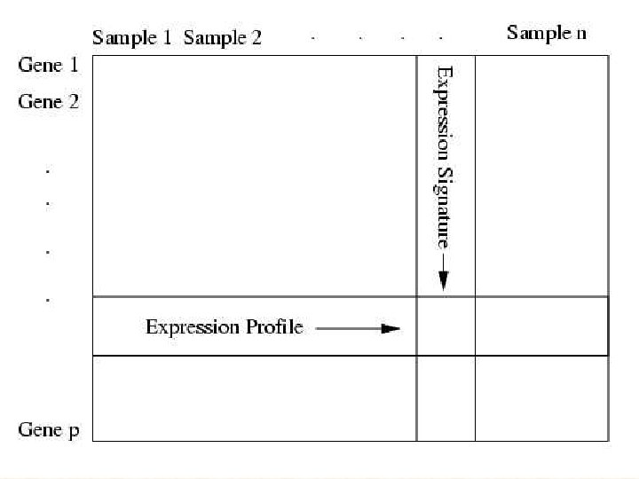
AIM: To link gene-expression data with survival from lung cancer A. CLUSTER ANALYSIS. We apply a model-based clustering approach to classify tumor tissues on the basis of microarray gene expression. The impact of this classification on cancer biology and clinical outcome is studied. B. SURVIVAL ANALYSIS. The association between the clusters so formed and patient survival (recurrence) times is examined. C. DISCRIMINANT ANALYSIS. We show that the prognosis clustering is a more powerful predictor of the outcome of disease than current systems based on histopathology criteria and extent of disease at presentation.

STANFORD and ONTARIO DATASETS: Both these datasets include tissues of various tumor types, as shown in Table 1. The major differences in samples are that the Stanford Dataset contains relatively more adenocarcinoma (AC) samples, and the Ontario Dataset contains only non-small cell carcinomas (NSCLC). In both studies c. DNA microarrays were used to obtain gene expression profiles for the tissue (tumour) samples. STANFORD: 918 genes ONTARIO: 2880 genes

Initial Gene Selection We start with the reduced datasets; the Stanford subset of 918 genes (with most similar expression within tumor pairs, but which differed among the other tumor samples) and the Ontario subset of 2880 genes (which contained data points in at least 80 percent of the samples and the transcripts had at least two samples with an absolute value of two in log 2 space). The Stanford Dataset had a total of 73 samples (including matched samples), and the Ontario Dataset had a total of 39 samples.

Table 1. Comparison of Tumor Types for Stanford and Ontario Datasets

MIXTURE OF g NORMAL COMPONENTS where constant MAHALANOBIS DISTANCE EUCLIDEAN DISTANCE

MIXTURE OF g NORMAL COMPONENTS k-means SPHERICAL CLUSTERS

With a mixture model-based approach to clustering, an observation is assigned outright to the ith cluster if its density in the ith component of the mixture distribution (weighted by the prior probability of that component) is greater than in the other (g-1) components.

Mixtures of Factor Analyzers A normal mixture model without restrictions on the component-covariance matrices may be viewed as too general for many situations in practice, in particular, with high dimensional data. One approach for reducing the number of parameters is to work in a lower dimensional space by adopting mixtures of factor analyzers.

Bi is a p x q matrix and Di is a diagonal matrix.

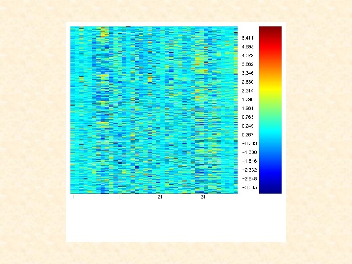
Liat , can you please add some legends to the following heat map.

CLUSTERING OF ONTARIO TUMOURS Using EMMIX-GENE Steps used in the application of EMMIX-GENE: 1. Select the most relevant genes from this filtered set of 2, 880 genes. The set of retained genes is thus reduced to 766. 2. Cluster these 766 genes into twenty groups. The majority of gene groups produced were reasonably cohesive and distinct. 3. Using these twenty group means, cluster the tissue samples into two groups using a mixture of normal components/factor analyzers.

Genes Heat Maps for the 20 Ontario Gene Groups Tissues are ordered as: Recurrence (1 -24) and Censored (25 -39)

Expression Profiles for Useful Metagenes (Ontario 39 Tissues) Gene Group 1 Gene Group 2 Log Expression Value Our Tissue Cluster 1 Our Tissue Cluster 2 Recurrence (1 -24) Censored (25 -39) Gene Group 19 Gene Group 20 Tissues

Selection of Relevant Genes We retain only 1 of the 16 genes of interest mentioned in the Ontario study (ZNF 136). Why are the others rejected by us yet retained in the Ontario study?

Expression Profiles of some Genes Identified in Ontario Cluster A Clusters B and C Log Expression Value (down Rec, up Censored) PNUTL 1 Recurrence (1 -24) (up Rec, down Censored) ATM Censored (25 -39) Recurrence (1 -24) FUS HIF 1 A Wee 1 RABIF Censored (25 -39) Tissues

Log Expression Value Only ZNF 136 is retained by us and also identified in Ontario Tissues Recurrence (1 -24) Censored (25 -39) It is found in our Group 19 (up-regulated in recurrence).

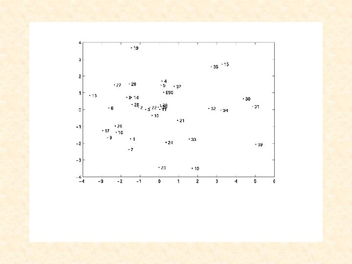
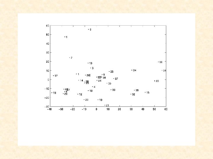
Tumours 1 -24 belong to RECURRENCE group Tumours 25 -39 are censored CLUSTER ANALYSIS via EMMIX-GENE of 20 METAGENES yields TWO CLUSTERS: CLUSTER 1: 1 -14, 16 -24 (recurrence) plus 25 -29, 33, 36, 38 (censored) CLUSTER 2: 15 (recurrence) plus 30 -32, 34, 35, 37, 39 (censored)

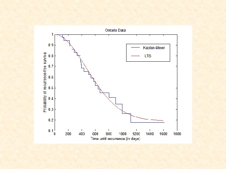
SURVIVAL ANALYSIS: LONG-TERM SURVIVAL (LTS) MODEL where T is time to recurrence and p 1 = 1 - p 2 is the prior prob. of recurrence. Adopt Weibull model for the survival function for recurrence S 1(t).

Liat, can you add a title and x- and y-legends to the next slide: Title: PCA of Tissues Based on Metagenes X-axis: First PC Y-axis: Second PC

Liat, can you add a title and x- and y-legends to the next slide: Title: PCA of Tissues Based on All Genes (via SVD) X-axis: First PC Y-axis: Second PC

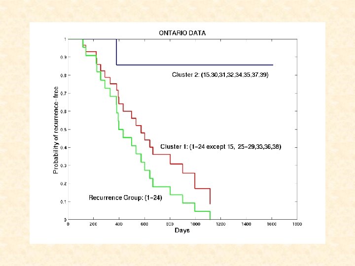
Survival Analysis for Ontario Dataset • Kaplan-Meier estimation: Cluster 1 2 No. of Tissues No. of Censored 29 8 Mean time to Failure ( SE) 665 85. 9 1388 155. 7 8 7 A significant difference in recurrence-free between clusters (P=0. 027) • Cox’s proportional hazards analysis: Variable Cluster 1 vs. Cluster 2 Tumor stage Hazard ratio (95% CI) P-value 6. 78 (0. 9 – 51. 5) 1. 07 (0. 57 – 2. 0) 0. 06 0. 83

Supervised Classification Method Based on a supervised clustering approach, a prognosis classifier was developed to predict the class of origin of a tumor tissue with a small error rate after correction for the selection bias. A support vector machine (SVM) was adopted to identify important genes that play a key role on predicting the clinical outcome, using all the genes, and the metagenes. A cross-validation (CV) procedure was then performed to calculate the test error, after corrected for the selection bias.

ONTARIO DATA (39 tissues): Support Vector Machine (SVM) with Recursive Feature Elimination (RFE) 0. 12 Error Rate (CV 10 E) 0. 1 0. 08 0. 06 0. 04 0. 02 0 0 2 4 6 8 10 12 log 2 (number of genes) Ten-fold Cross-Validation Error Rate (CV 10 E) of Support Vector Machine (SVM). applied to g=2 clusters (G 1: 1 -14, 16 - 29, 33, 36, 38; G 2: 15, 30 -32, 34, 35, 37, 39)

Genes Heat Maps for the 20 Stanford Gene Clusters (73 Tissues) Tissues are ordered by their histological classification: Adenocarcinoma (1 -41), Fetal Lung (42), Large cell (43 -47), Normal (48 -52), Squamous cell (53 -68), Small cell (69 -73)

Genes Heat Maps for the 15 Stanford Gene Clusters (35 Tissues) Tissues are ordered by the Stanford classification into AC groups: AC group 1 (1 -19), AC group 2 (20 -26), AC group 3 (27 -35)

Expression Profiles for Top Metagenes (Stanford 35 AC Tissues) Log Expression Value Gene Group 1 Gene Group 2 Stanford AC group 1 Stanford AC group 2 Stanford AC group 3 Misallocated Gene Group 3 Gene Group 4 Tissues

Some other interesting Metagenes Gene Group 9 Log Expression Value Gene Group 7 Tissues Group 7 (19 genes) includes: Group 9 (22 genes) includes: citron surfactant A 1 ICAM-1 (CD 54) collagen, type IX hepsin thyroid transcription factor Marker Genes For Group 1 (Supervised) High in group 1, low in 2 (1/ 9 genes) Surfactant Proteins (Unsupervised) High in groups 1 and 2, low in 3 Marker Genes For Group 1 (Supervised) High in group 1, low in 2 (4/ 9 genes)

Which Genes make up the top 4 Metagenes ? Group 1 (22 genes) includes: Group 2 (12 genes) includes: ESTs Hs. 11607 ataxia-telangiectasia group D-associated protein solute carrier family 7, member 5 (CD 98) vascular endothelial growth factor C ornithine decarboxylase carbonyl reductase (metabolic enzyme) Marker Genes For Group 3 (Supervised) Marker Genes for Group 2 (Supervised) High in group 3, low in 1 and 2 (4/10 genes) High in group 2, low in 3 (1/8 genes) Group 3 (16 genes) includes: Group 4 (14 genes) includes: aldo-keto reductase family 1 glutathione peroxidase thioredoxin reductase cartilage paired-class homeoprotein tumor suppressor deleted in oral cancer-related 1 Metabolic Enzymes (Unsupervised) Marker Genes for Group 2 (Supervised) High in group 3, also SCC (3/6 genes) High in group 2, low in 3 (2/8 genes)

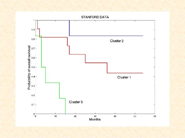
STANFORD DATA: Cluster 1: 1 -19 (good prognosis) Cluster 2: 20 -26 (long-term survivors) Cluster 3: 27 -35 (poor prognosis)

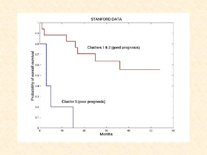
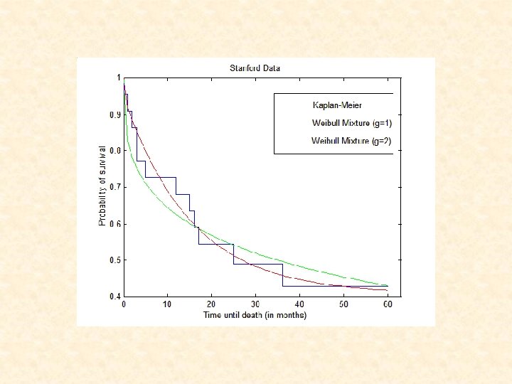
STANFORD DATA: TWO-COMPONENT WEIBULL MIXTURE MODEL where

Survival Analysis for Stanford Dataset • Kaplan-Meier estimation: Cluster 1 2 No. of Tissues No. of Censored 17 5 Mean time to Failure ( SE) 37. 5 5. 0 5. 2 2. 3 10 0 A significant difference in survival between clusters (P<0. 001) • Cox’s proportional hazards analysis: Variable Cluster 2 vs. Cluster 1 Grade 3 vs. grades 1 or 2 Tumor size No. of tumors in lymph nodes Presence of metastases Hazard ratio (95% CI) P-value 13. 2 (2. 1 – 81. 1) 1. 94 (0. 5 – 8. 5) 0. 96 (0. 3 – 2. 8) 1. 65 (0. 7 – 3. 9) 4. 41 (1. 0 – 19. 8) 0. 005 0. 38 0. 93 0. 25 0. 05

Survival Analysis for Stanford Dataset • Univariate Cox’s proportional hazards analysis (metagenes): Metagene Coefficient (SE) P-value 1 2 3 4 5 1. 37 (0. 44) -0. 24 (0. 31) 0. 14 (0. 34) -1. 01 (0. 56) 0. 66 (0. 65) 0. 002 0. 44 0. 68 0. 07 0. 31 6 7 8 9 10 -0. 63 (0. 50) -0. 68 (0. 57) 0. 75 (0. 46) -1. 13 (0. 50) 0. 73 (0. 39) 0. 20 0. 24 0. 10 0. 02 0. 06 11 12 13 14 15 0. 35 (0. 50) -0. 55 (0. 41) -0. 61 (0. 48) 0. 22 (0. 36) 1. 70 (0. 92) 0. 48 0. 18 0. 20 0. 53 0. 06

Survival Analysis for Stanford Dataset • Multivariate Cox’s proportional hazards analysis (metagenes): Metagene Coefficient (SE) P-value 1 3. 44 (0. 95) 0. 0003 2 -1. 60 (0. 62) 0. 010 8 -1. 55 (0. 73) 0. 033 11 1. 16 (0. 54) 0. 031 The final model consists of four metagenes.

STANFORD DATA: Support Vector Machine (SVM) with Recursive Feature Elimination (RFE) 0. 07 Error Rate (CV 10 E) 0. 06 0. 05 0. 04 0. 03 0. 02 0. 01 0 0 1 2 3 4 5 6 7 8 9 10 log 2 (number of genes) Ten-fold Cross-Validation Error Rate (CV 10 E) of Support Vector Machine (SVM). Applied to g=2 clusters.

MICHIGAN DATA 4965 genes on 86 AC tumours (oligonucleotide arrays) We imposed a floor of – 100; ceiling of 26, 000; applied generalized log transformation, and then row normalized but not column normalized

Genes Heat Maps for the 40 Michigan Gene Groups Tissues in order of our clusters: Cluster 1 (1 -34) Cluster 2 (35 -69) Cluster 3 (70 -86) Tissues

MICHIGAN DATA: LTS MODEL where CONCLUDE:

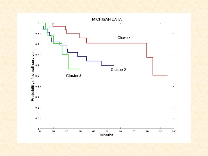
Survival Analysis for Michigan Dataset • Kaplan-Meier estimation: Cluster No. of Tissues No. of Censored Mean time to Failure ( SE) 1 2 3 34 35 17 27 23 12 84. 1 7. 3 73. 5 8. 5 41. 7 7. 8 No significant difference in survival between clusters • Long-term survivor model: Estimates (SE) S 1(t) (Weibull distribution) a : 0. 017 (0. 007); b : 1. 116 (0. 215) p 2 (Logistic function) -0. 712 (0. 218); 0. 654 (0. 169); 0. 723 (0. 702) A significant difference in p 2 between Clusters 1 & 2 Proportion of long-term survivors Cluster 1 Cluster 2 Cluster 3 67. 1% 51. 5% 34. 0%

MICHICAN DATA: Support Vector Machine (SVM) with Recursive Feature Elimination (RFE) applied to g=3 clusters Error Rate (CV 10 E) 0. 5 0. 4 0. 3 0. 2 0. 1 0 0 2 4 6 8 10 12 14 log 2 (number of genes) Ten-fold Cross-Validation Error Rate (CV 10 E) of Support Vector Machine (SVM) applied to 3 clusters.

HARVARD DATA: genes on 203 AC tumours (oligonucleotide arrays) We impose a floor of – 1; ceiling of 3, 000; logged data and then column and row normalized

Genes Heat Maps for the 20 Harvard Gene Groups (126 tissues) Tissues are ordered as our clusters: Cluster 1 (1 -53), Cluster 2 (54 -126) Tissues

Genes Heat Maps for the 20 Harvard Gene Groups (126 tissues) Tissues are ordered as our clusters: Cluster 1 (1 -55), Cluster 2 (56 -110), Cluster 3 (111 -126)

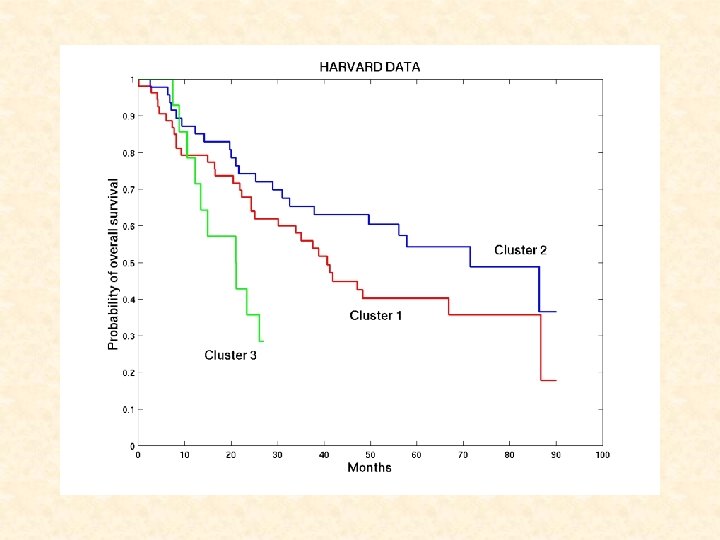
Survival Analysis for Harvard Dataset • Kaplan-Meier estimation: Cluster 1 2 3 No. of Tissues No. of Censored 54 47 14 Mean time to Failure ( SE) 50. 9 5. 8 62. 2 5. 7 26. 5 4. 7 22 25 4 A significant difference in survival between clusters (P=0. 044) • Cox’s proportional hazards analysis: Variable Cluster 2 vs. Cluster 1 Cluster 3 vs. Cluster 2 Age Female vs. Male Smoking frequency Tumor size Presence of tumor in lymph nodes Stage Hazard ratio (95% CI) P-value 0. 74 (0. 4 – 1. 4) 3. 08 (1. 4 – 6. 8) 1. 02 (1. 0 – 1. 1) 0. 56 (0. 3 – 1. 0) 1. 24 (0. 6 – 2. 5) 1. 68 (0. 9 – 3. 3) 2. 50 (1. 3 – 4. 8) 1. 43 (0. 7 – 2. 9) 0. 34 0. 005 0. 12 0. 06 0. 54 0. 13 0. 006 0. 33

HARVARD DATA: Support Vector Machine (SVM) with Recursive Feature Elimination (RFE) applied to g=2 clusters 0. 1 0. 09 Error Rate (CV 10 E) 0. 08 0. 07 0. 06 0. 05 0. 04 0. 03 0. 02 0. 01 0 0 1 2 3 4 log 2 (number of genes) Ten-fold Cross-Validation Error Rate (CV 10 E) of Support Vector Machine (SVM) applied to 2 clusters.

? ? ? ? ? ? ? ? ? ? ? ? ? ? There are some obstacles to integrate information from the Stanford and Ontario Datasets. In the Stanford Dataset, we have clinical data only for the adenocarcinoma (plus two other) samples that are classified into their AC groupings. On the other hand, in the Ontario Dataset we have clinical data for various tumor types. The Ontario study attempts to relate non-adenocarcinoma samples, as well as adenocarcinoma samples, to clinical outcome. In order to do so, they simply cluster the tumors into two groups; recurrence vs non-recurrence, with no evidence for adenocarcinoma subclasses as found in the Stanford study. Additionally, within our gene clusters, we could not find genes common to both datasets.

CONCLUSIONS ? ? ? ? ? ? ? ? ? ? We developed a model-based clustering approach to classify tumor tissues using microarrays genes expression profile. The clustering performed best as a predictor of the clinical outcome based on the overall survival or recurrence times. The results obtained from the analysis of both Stanford and Ontario Datasets indicate that classification of patients into goodprognosis and poor-prognosis subgroups on the basis of microarrays could be a useful tool for linking the impact on lung cancer biology and guiding treatment therapy and patient care to lung cancer patients.

ACKNOWLEDGMENTS We thank colleagues: Nazim Khan Abdollah Khodkar Justin Zhu.