Use of genomic recursions in singlestep genomic best

Use of genomic recursions in singlestep genomic best linear unbiased predictor (BLUP) with a large number of genotypes Dr. Breno Fragomeni Assistant Professor Animal Science - UConn

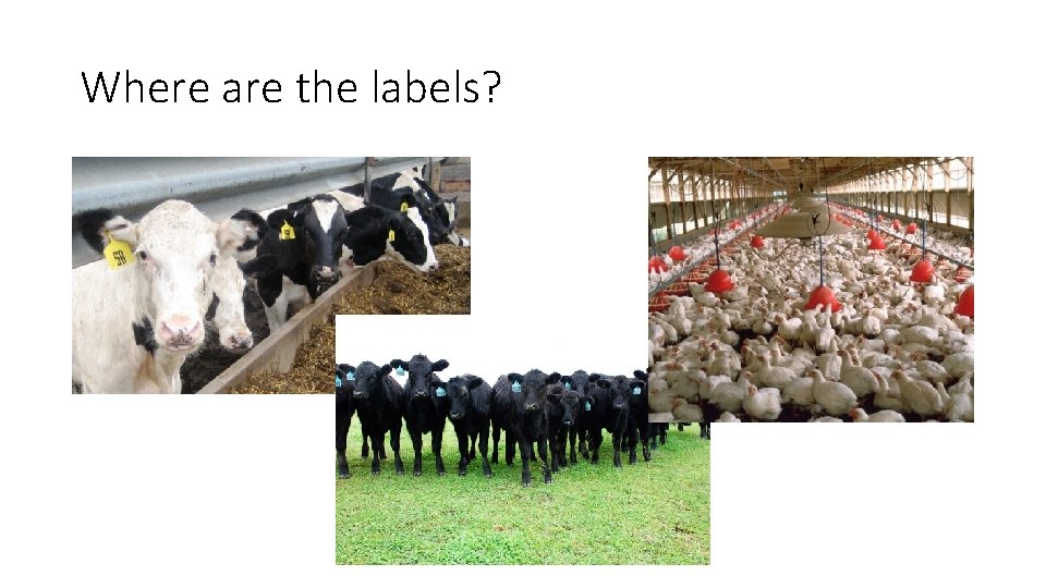
Where are the labels?

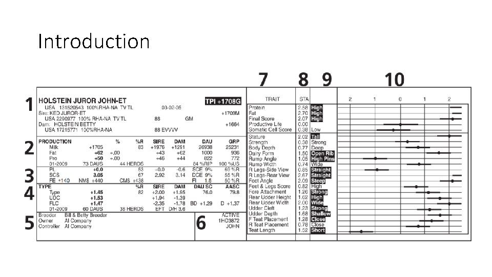
Introduction

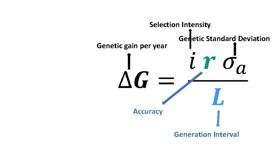
Selection Intensity Why genomic prediction? Genetic gain per year Genetic Standard Deviation • Higher accuracy • Shorter generation interval • Higher genetic gain Accuracy Generation Interval

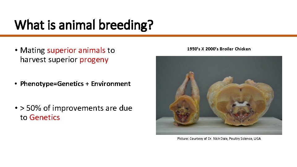
What is animal breeding? • Mating superior animals to harvest superior progeny 1950’s X 2000’s Broiler Chicken • Phenotype=Genetics + Environment • > 50% of improvements are due to Genetics Picture: Courtesy of Dr. Nick Dale, Poultry Science, UGA

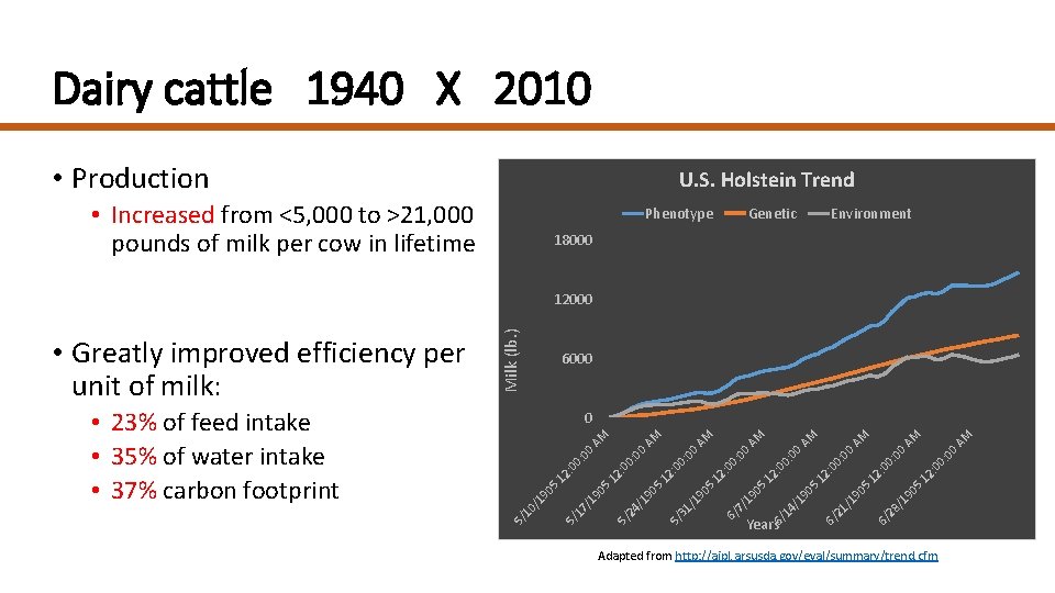
Dairy cattle 1940 X 2010 • Production U. S. Holstein Trend • Increased from <5, 000 to >21, 000 pounds of milk per cow in lifetime Phenotype Genetic Environment 18000 00 0: : 0 12 5 6/ 28 /1 90 90 /1 21 6/ A M M A 00 : 0 12 5 90 /1 14 6/ Years 0: 00 0: : 0 00 2: 1 05 19 7/ 6/ A M AM : 0 00 0: : 0 12 5 90 /1 31 5/ 0 A M 00 0: : 0 12 5 90 /1 5/ 24 90 /1 17 5/ /1 90 5 5 12 12 : 0 0: 00 00 A M 0 10 • 23% of feed intake • 35% of water intake • 37% carbon footprint 6000 5/ • Greatly improved efficiency per unit of milk: Milk (lb. ) 12000 Adapted from http: //aipl. arsusda. gov/eval/summary/trend. cfm

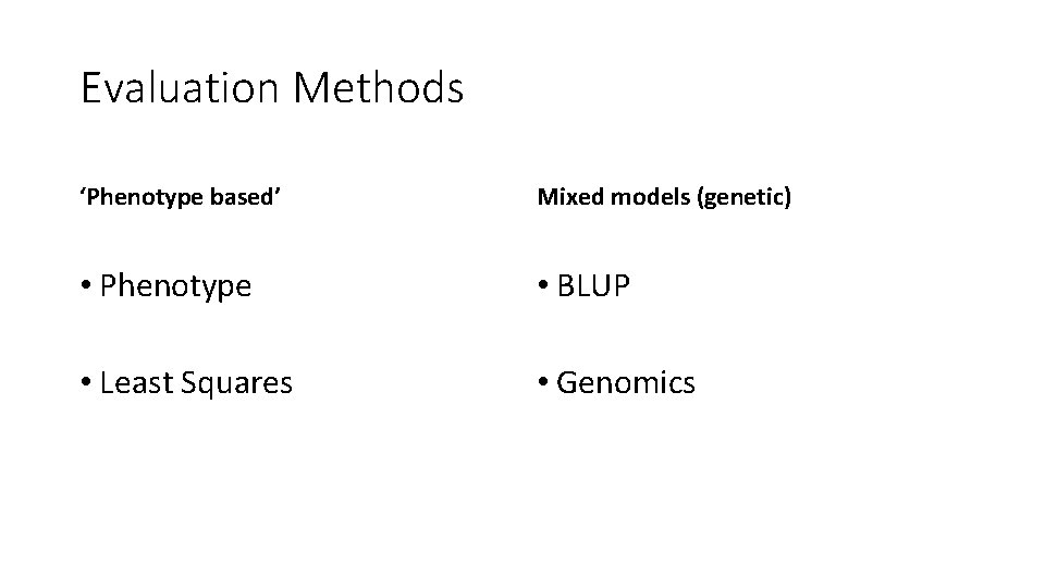
Evaluation Methods ‘Phenotype based’ Mixed models (genetic) • Phenotype • BLUP • Least Squares • Genomics

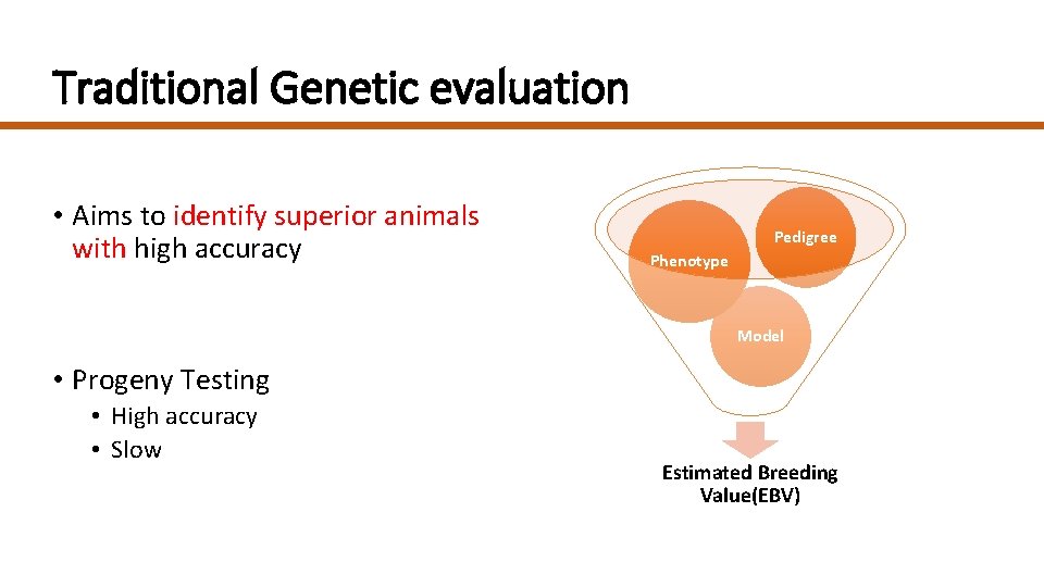
Traditional Genetic evaluation • Aims to identify superior animals with high accuracy Pedigree Phenotype Model • Progeny Testing • High accuracy • Slow Estimated Breeding Value(EBV)

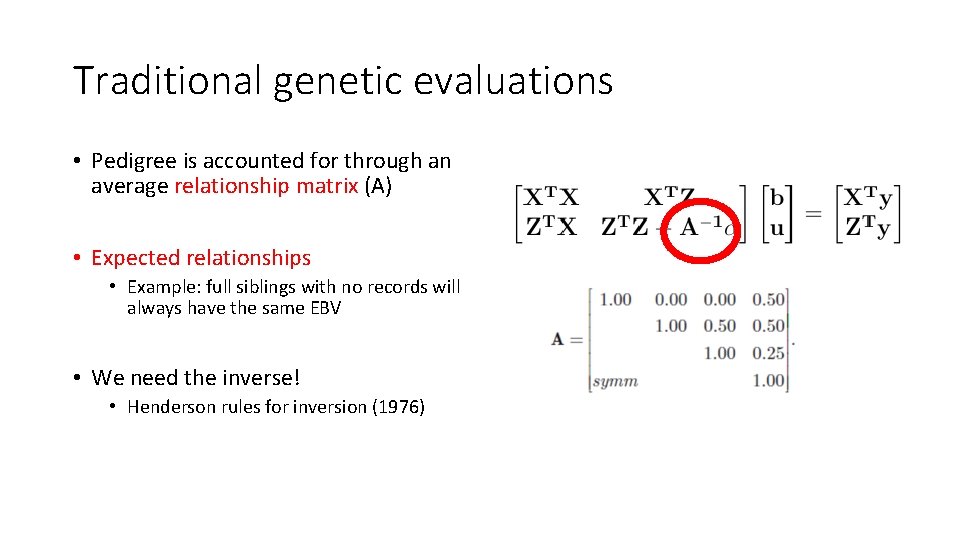
Traditional genetic evaluations • Pedigree is accounted for through an average relationship matrix (A) • Expected relationships • Example: full siblings with no records will always have the same EBV • We need the inverse! • Henderson rules for inversion (1976)

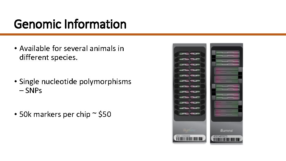
Genomic Information • Available for several animals in different species. • Single nucleotide polymorphisms – SNPs • 50 k markers per chip ~ $50

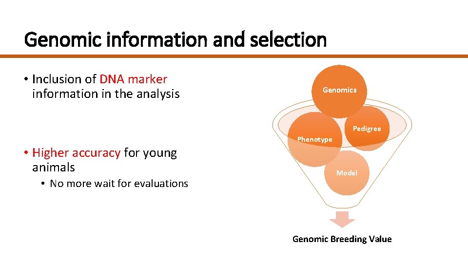
Genomic information and selection • Inclusion of DNA marker information in the analysis Genomics Pedigree • Higher accuracy for young animals • No more wait for evaluations Phenotype Model Genomic Breeding Value

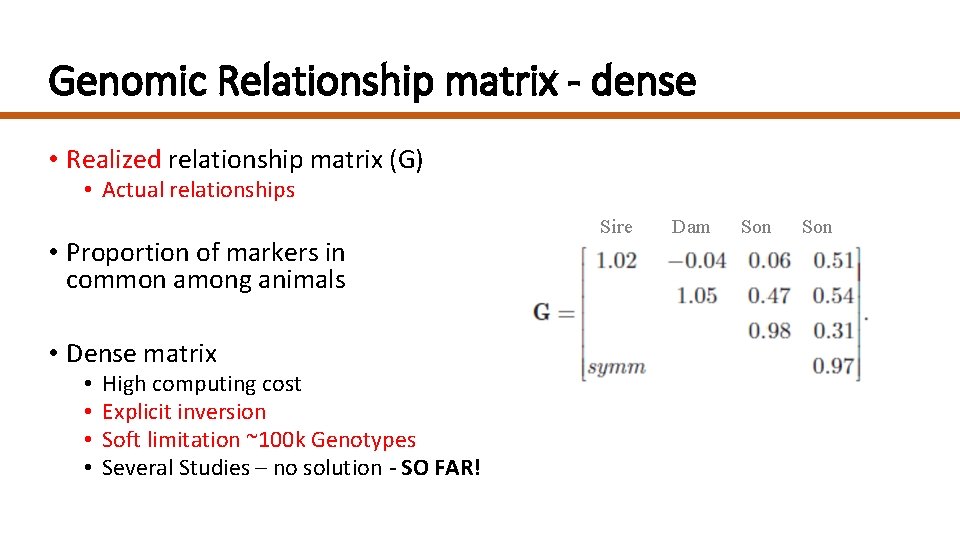
Genomic Relationship matrix - dense • Realized relationship matrix (G) • Actual relationships • Proportion of markers in common among animals • Dense matrix • • High computing cost Explicit inversion Soft limitation ~100 k Genotypes Several Studies – no solution - SO FAR! Sire Dam Son

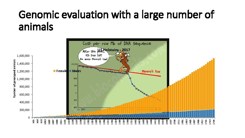
0 1705 1703 1701 1611 1609 1607 1605 1603 1601 1511 1509 1507 1505 1503 1501 1411 1409 1407 1405 1403 1401 1311 1309 1307 1305 1303 1301 1211 1209 1207 1205 1203 1201 1111 1109 1107 Females 1105 1103 1101 1011 1, 200, 000 1009 1007 1005 1002 910 906 901 Number of genotyped animals Genomic evaluation with a large number of animals US Holsteins - 2017 1, 600, 000 1, 400, 000 Males 1, 000 800, 000 600, 000 400, 000 200, 000

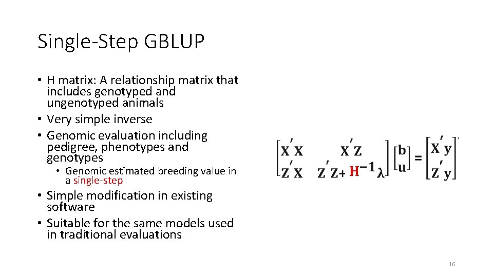
Single-Step GBLUP • H matrix: A relationship matrix that includes genotyped and ungenotyped animals • Very simple inverse • Genomic evaluation including pedigree, phenotypes and genotypes • Genomic estimated breeding value in a single-step H • Simple modification in existing software • Suitable for the same models used in traditional evaluations 16

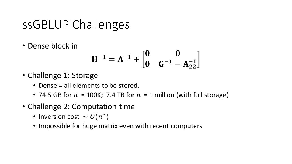
ss. GBLUP Challenges •

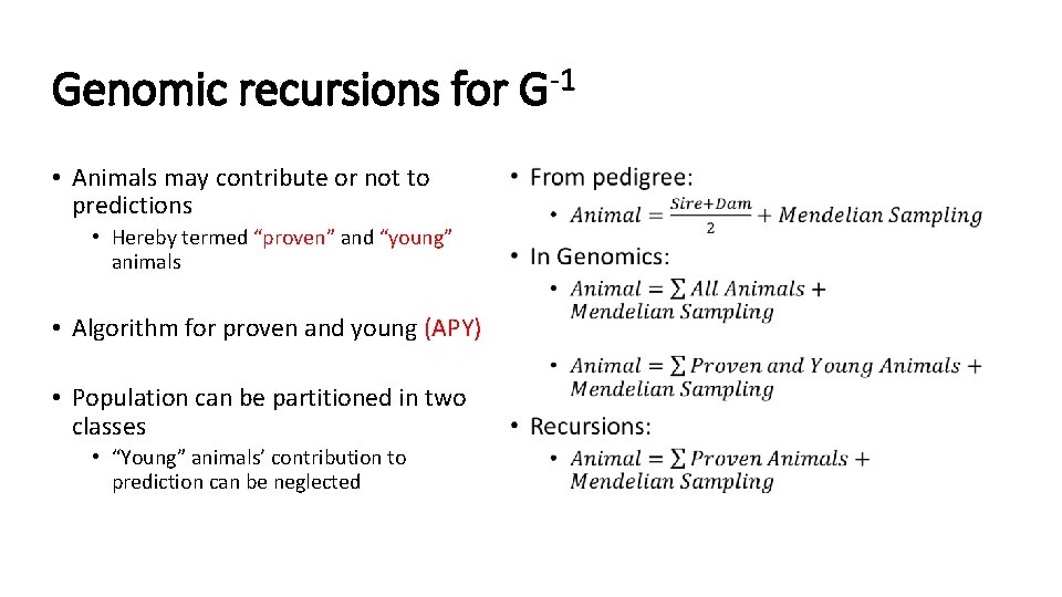
Genomic recursions for G-1 • Animals may contribute or not to predictions • Hereby termed “proven” and “young” animals • Algorithm for proven and young (APY) • Population can be partitioned in two classes • “Young” animals’ contribution to prediction can be neglected •

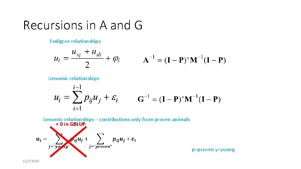
Recursions in A and G Pedigree relationships Genomic relationships – contributions only from proven animals = 0 in GBLUP p=proven y=young 10/7/2020

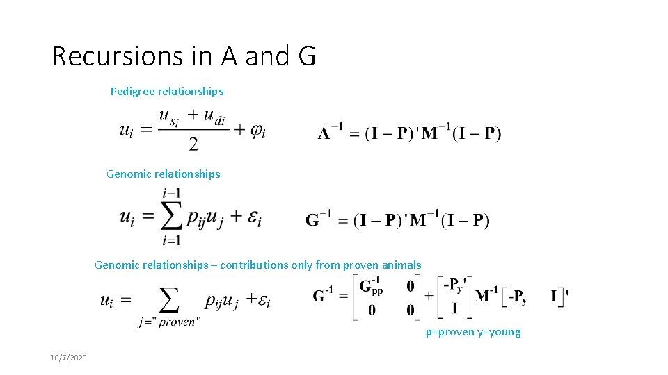
Recursions in A and G Pedigree relationships Genomic relationships – contributions only from proven animals p=proven y=young 10/7/2020

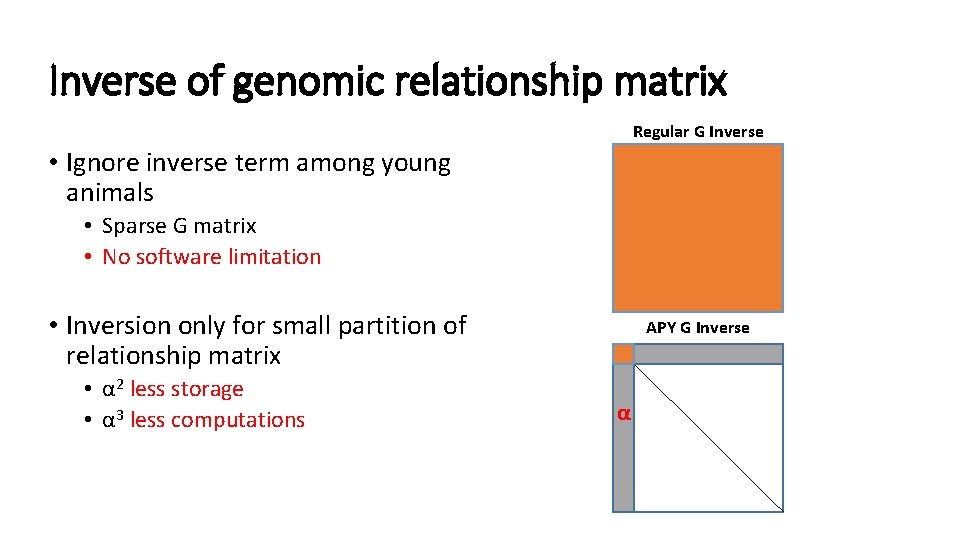
Inverse of genomic relationship matrix Regular G Inverse • Ignore inverse term among young animals • Sparse G matrix • No software limitation • Inversion only for small partition of relationship matrix • α 2 less storage • α 3 less computations APY G Inverse α

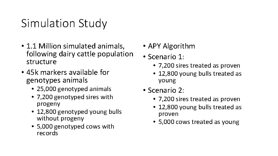
Simulation Study • 1. 1 Million simulated animals, • APY Algorithm following dairy cattle population • Scenario 1: structure • 7, 200 sires treated as proven • 45 k markers available for • 12, 800 young bulls treated as young genotypes animals • 25, 000 genotyped animals • Scenario 2: • 7, 200 genotyped sires with progeny • 12, 800 genotyped young bulls without progeny • 5, 000 genotyped cows with records • 7, 200 sires treated as proven • 12, 800 young bulls treated as proven • 5, 000 cows treated as young

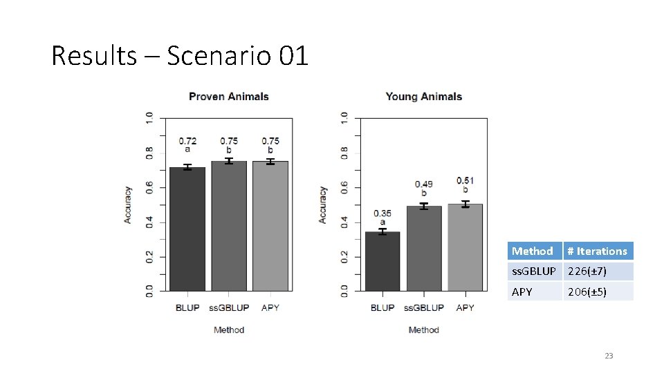
Results – Scenario 01 Method # Iterations ss. GBLUP 226(± 7) APY 206(± 5) 23

Results - Scenario 02 Method # Iterations ss. GBLUP 231(± 7) APY 209(± 6) 24

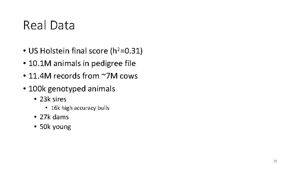
Real Data • US Holstein final score (h 2=0. 31) • 10. 1 M animals in pedigree file • 11. 4 M records from ~7 M cows • 100 k genotyped animals • 23 k sires • 16 k high accuracy bulls • 27 k dams • 50 k young 25

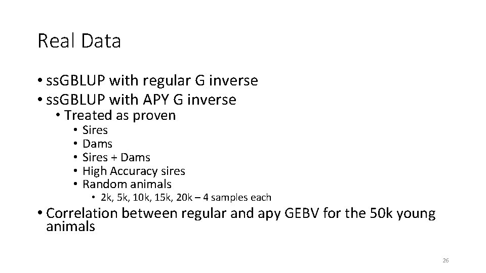
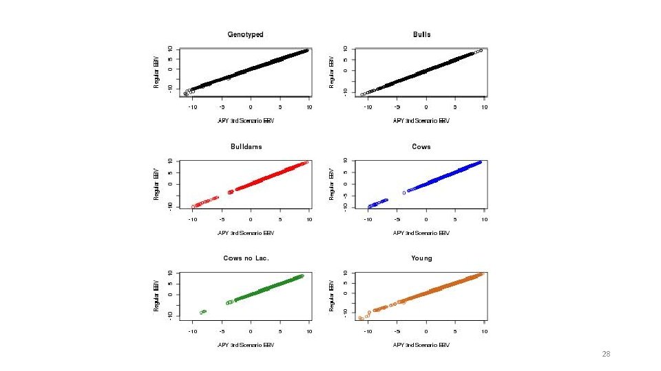
Real Data • ss. GBLUP with regular G inverse • ss. GBLUP with APY G inverse • Treated as proven • • • Sires Dams Sires + Dams High Accuracy sires Random animals • 2 k, 5 k, 10 k, 15 k, 20 k – 4 samples each • Correlation between regular and apy GEBV for the 50 k young animals 26

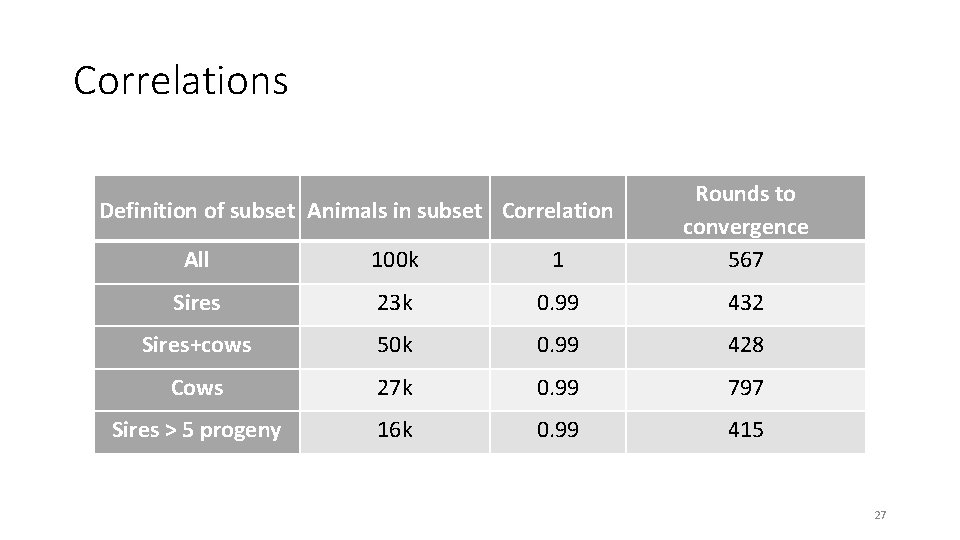
Correlations All 100 k 1 Rounds to convergence 567 Sires 23 k 0. 99 432 Sires+cows 50 k 0. 99 428 Cows 27 k 0. 99 797 Sires > 5 progeny 16 k 0. 99 415 Definition of subset Animals in subset Correlation 27

28

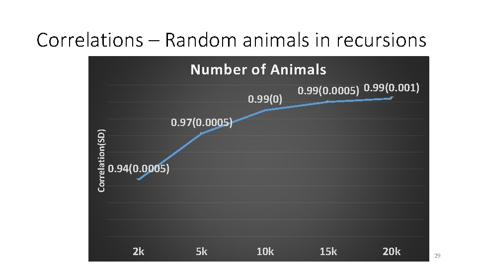
Correlations – Random animals in recursions Number of Animals Correlation(SD) 0. 99(0. 0005) 0. 99(0. 001) 0. 97(0. 0005) 0. 94(0. 0005) 2 k 5 k 10 k 15 k 20 k 29

Implications • Academic • New understanding of genomic dimensionality • Industry • Limitation is over: genomic selection for millions of animals • New area of research • Interest from groups all over the • Companies and breed world associations are adopting the method

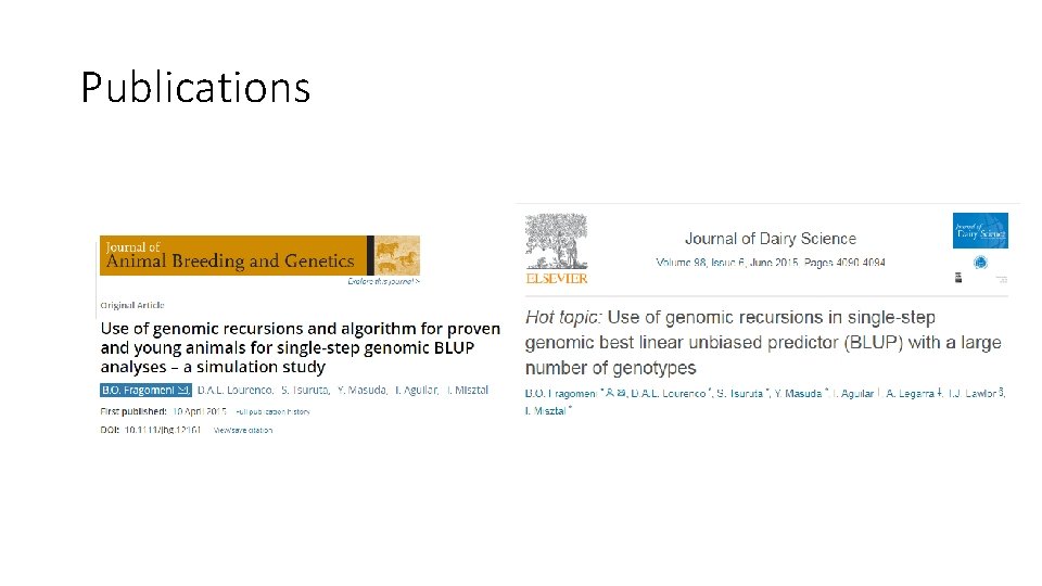
Publications