Use of Autocorrelation Kernels in Kernel Canonical Correlation

Use of Autocorrelation Kernels in Kernel Canonical Correlation Analysis for Texture Classification Yo Horikawa Kagawa University , Japan 1

･Support vector machine (SVM) ･Kernel canonical correlation analysis (k. CCA) 　with autocorrelation kernels → Invariant texture classification only using raw pixel data without explicit feature extraction Compare the performance of the kernel methods. Discuss the effects of the order of autocorrelation kernels. 2

Support vector machine (SVM) Sample data: xi (1 ≤ i ≤ n), belonging to Class ci ∊ {-1, 1} SVM learns a discriminant function for test data x: d(x) = sgn(∑i=1 n’ αici. K(x, xsi) + b) αi and b are obtained through the quadratic programming problem. Kernel function: Inner product of nonlinear maps φ(x): K(xi, xj) = φ(xi)･φ(xj) Support vectors: xsi (1 ≤ i ≤ n’ (≤ n)): a part of sample data Feature extraction process is implicitly done in SVM through the kernel function and support vectors. 3

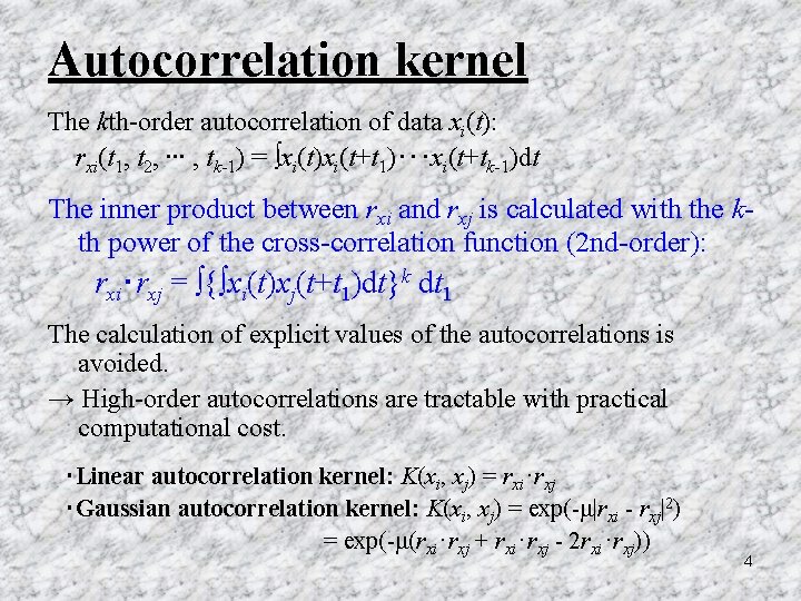
Autocorrelation kernel The kth-order autocorrelation of data xi(t): rxi(t 1, t 2, ∙∙∙ , tk-1) = ∫xi(t)xi(t+t 1)･･･xi(t+tk-1)dt The inner product between rxi and rxj is calculated with the kth power of the cross-correlation function (2 nd-order): rxi･rxj = ∫{∫xi(t)xj(t+t 1)dt}k dt 1　 The calculation of explicit values of the autocorrelations is avoided. → High-order autocorrelations are tractable with practical computational cost. 　･Linear autocorrelation kernel: K(xi, xj) = rxi･rxj 　･Gaussian autocorrelation kernel: K(xi, xj) = exp(-μ|rxi - rxj|2) = exp(-μ(rxi･rxj + rxi･rxj - 2 rxi･rxj)) 4

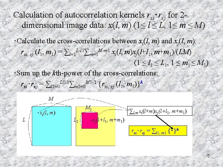
Calculation of autocorrelation kernels rxi･rxj for 2 dimensional image data: x(l, m) (1≤ l ≤ L, 1≤ m ≤ M) ･Calculate the cross-correlations between xi(l, m) and xj(l, m): rxi, xj (l 1, m 1) = ∑l=1 L-l 1∑m=1 M-m 1 xi(l, m)xj(l+l 1, m+m 1)/(LM) (1 ≤ l 1 ≤ L 1, 1 ≤ m 1 ≤ M 1) ･Sum up the kth-power of the cross-correlations: rxi･rxj = ∑l 1=0 L 1 -1∑m 1=0 M 1 -1 {rxi, xj (l 1, m 1)}k M L xi(l, m) M 1 L 1 ∑l, m xi(l+m)xj(l+l 1, m+m 1) rxi･rxj = ∑l 1, m 1 {・}k 5

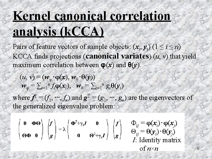
Kernel canonical correlation analysis (k. CCA) Pairs of feature vectors of sample objects: (xi, yi) (1 ≤ i ≤ n) KCCA finds projections (canonical variates) (u, v) that yield maximum correlation between φ(x) and θ(y). (u, v) = (wφ･φ(x), wθ･θ(y)) wφ = ∑i=1 n fiφ(xi), wθ = ∑i=1 n giθ(yi) where f. T = (f 1, ∙∙∙, fn) and g. T = (g 1, ∙∙∙, gn) are the eigenvectors of the generalized eigenvalue problem: Φij = φ(xi)･φ(xj) Θij = θ(yi)･θ(yj) I: Identity matrix 　　　　　　　of n×n 6

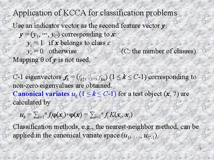
Application of KCCA for classification problems Use an indicator vector as the second feature vector y. y = (y 1, ∙∙∙, y. C) corresponding to x: yc = 1 if x belongs to class c yc = 0 otherwise (C: the number of classes) Mapping θ of y is not used. C-1 eigenvectors fk = (fk 1, …, fkn) (1 ≤ k ≤ C-1) corresponding to non-zero eigenvalues are obtained. Canonical variates uk (1 ≤ k ≤ C-1) for a test object (x, ? ) are calculated by uk = ∑i=1 n fiφ(xi)･φ(x) = ∑i=1 n fi K(xi, xj) Classification methods, e. g. , the nearest-neighbor method, can be applied in the canonical variate space (u 1, …, u. C-1). 7

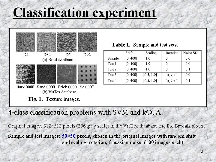
Classification experiment Table 1. Sample and test sets. Fig. 1. Texture images. 4 -classification problems with SVM and k. CCA Original images: 512× 512 pixels (256 gray scale) in the Vis. Tex database and the Brodatz album Sample and test images: 50× 50 pixels, chosen in the original images with random shift and scaling, rotation, Gaussian noise (100 images each) 8

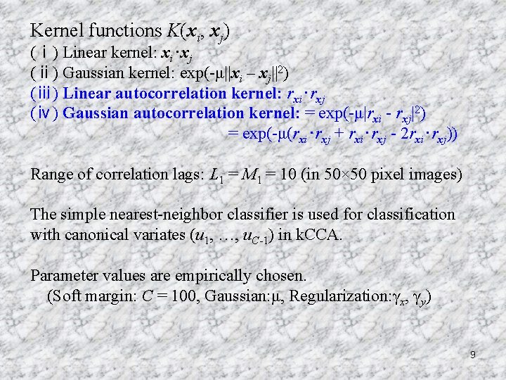
Kernel functions K(xi, xj) (ⅰ) Linear kernel: xi･xj (ⅱ) Gaussian kernel: exp(-μ||xi – xj||2) (ⅲ) Linear autocorrelation kernel: rxi･rxj　 (ⅳ) Gaussian autocorrelation kernel: = exp(-μ|rxi - rxj|2) = exp(-μ(rxi･rxj + rxi･rxj - 2 rxi･rxj)) Range of correlation lags: L 1 = M 1 = 10 (in 50× 50 pixel images) The simple nearest-neighbor classifier is used for classification with canonical variates (u 1, …, u. C-1) in k. CCA. Parameter values are empirically chosen. (Soft margin: C = 100, Gaussian: μ, Regularization: γx, γy) 9

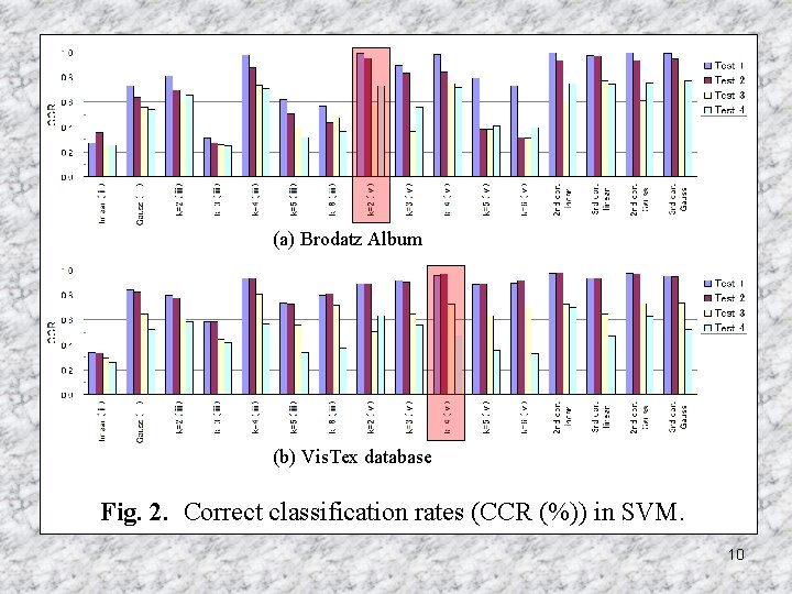
(a) Brodatz Album (b) Vis. Tex database Fig. 2. Correct classification rates (CCR (%)) in SVM. 10

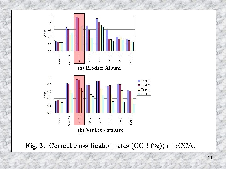
(a) Brodatz Album (b) Vis. Tex database Fig. 3. Correct classification rates (CCR (%)) in k. CCA. 11

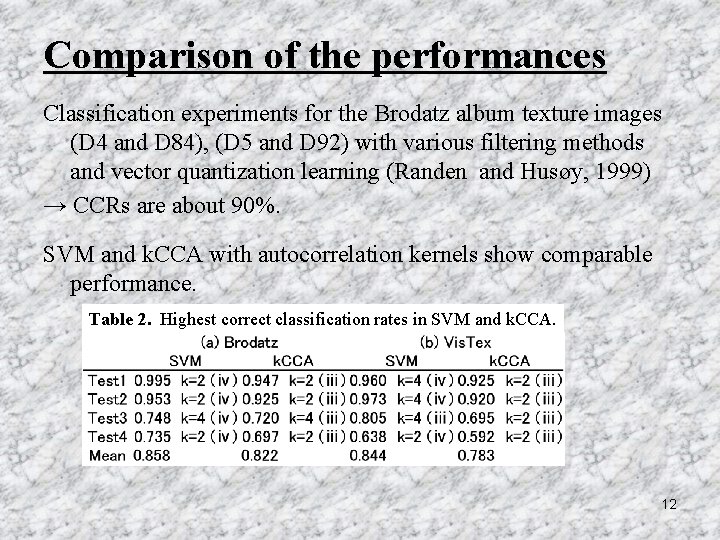
Comparison of the performances Classification experiments for the Brodatz album texture images (D 4 and D 84), (D 5 and D 92) with various filtering methods and vector quantization learning (Randen and Husøy, 1999) → CCRs are about 90%. SVM and k. CCA with autocorrelation kernels show comparable performance. Table 2. Highest correct classification rates in SVM and k. CCA. 12

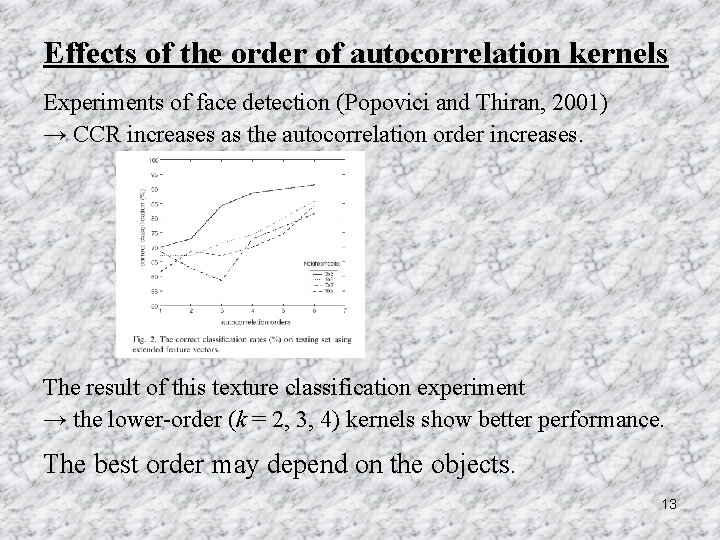
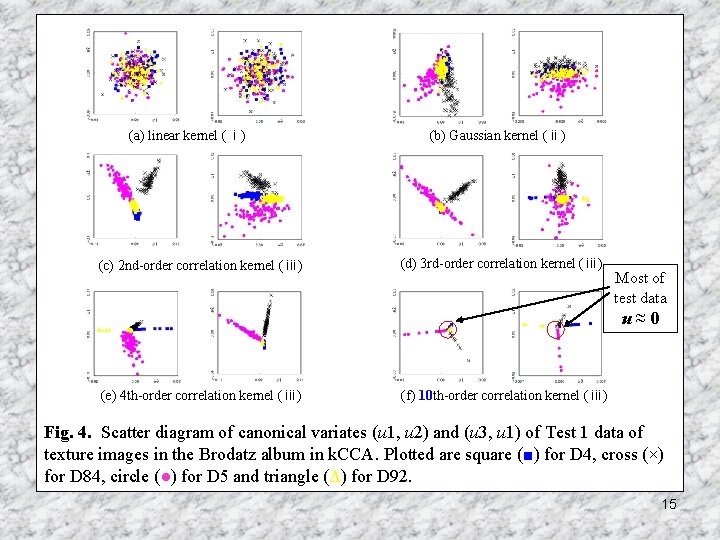
Effects of the order of autocorrelation kernels Experiments of face detection (Popovici and Thiran, 2001) → CCR increases as the autocorrelation order increases. The result of this texture classification experiment → the lower-order (k = 2, 3, 4) kernels show better performance. The best order may depend on the objects. 13

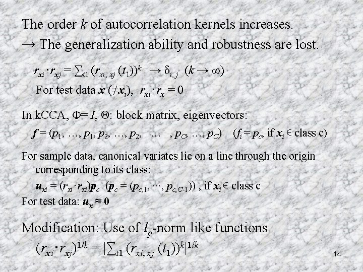
The order k of autocorrelation kernels increases. → The generalization ability and robustness are lost. rxi･rxj = ∑t 1 (rxi, xj (t 1))k → δi, j (k → ∞) For test data x (≠xi), rxi･rx = 0 In k. CCA, Φ= I, Θ: block matrix, eigenvectors: f = (p 1, …, p 1, p 2, … , p. C, …, p. C) (fi = pc, if xi ∊ class c) For sample data, canonical variates lie on a line through the origin corresponding to its class: uxi = (rxi･rxi)pc (pc = (pc, 1, ∙∙∙, pc, C-1)) , if xi ∊ class c For test data: ux ≈ 0 Modification: Use of lp-norm like functions (rxi･rxj)1/k = |∑t 1 (rxi, xj (t 1))k|1/k 14

(a) linear kernel (ⅰ) (c) 2 nd-order correlation kernel (ⅲ) (b) Gaussian kernel (ⅱ) (d) 3 rd-order correlation kernel (ⅲ) Most of test data u≈0 (e) 4 th-order correlation kernel (ⅲ) (f) 10 th-order correlation kernel (ⅲ) Fig. 4. Scatter diagram of canonical variates (u 1, u 2) and (u 3, u 1) of Test 1 data of texture images in the Brodatz album in k. CCA. Plotted are square (■) for D 4, cross (×) for D 84, circle (●) for D 5 and triangle (Δ) for D 92. 15

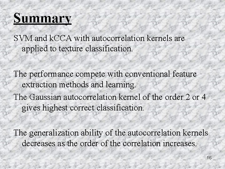
Summary SVM and k. CCA with autocorrelation kernels are applied to texture classification. The performance compete with conventional feature extraction methods and learning. The Gaussian autocorrelation kernel of the order 2 or 4 gives highest correct classification. The generalization ability of the autocorrelation kernels decreases as the order of the correlation increases. 16