US Army Logistics Management College Part 1 Simulation

US Army Logistics Management College Part 1: Simulation Modeling w/ Built in Excel Tools Simulation - 1

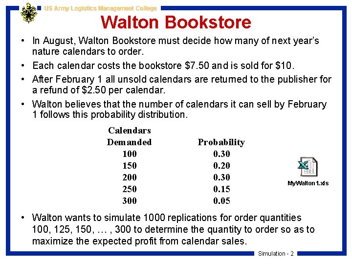
US Army Logistics Management College Walton Bookstore • In August, Walton Bookstore must decide how many of next year’s nature calendars to order. • Each calendar costs the bookstore $7. 50 and is sold for $10. • After February 1 all unsold calendars are returned to the publisher for a refund of $2. 50 per calendar. • Walton believes that the number of calendars it can sell by February 1 follows this probability distribution. Calendars Demanded 100 150 200 250 300 Probability 0. 30 0. 20 0. 30 0. 15 0. 05 My. Walton 1. xls • Walton wants to simulate 1000 replications for order quantities 100, 125, 150, … , 300 to determine the quantity to order so as to maximize the expected profit from calendar sales. Simulation - 2

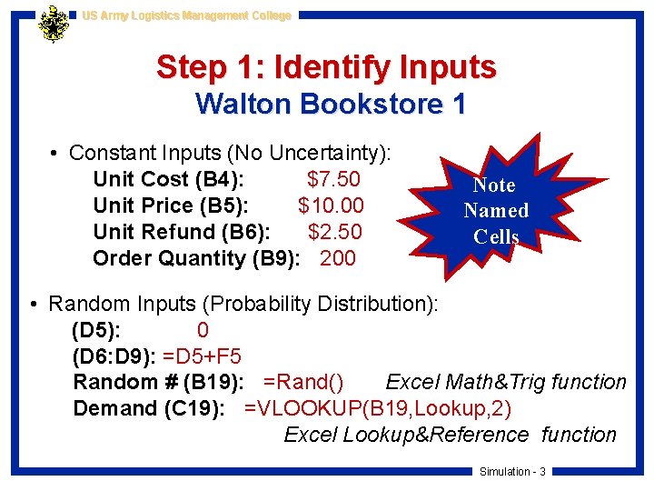
US Army Logistics Management College Step 1: Identify Inputs Walton Bookstore 1 • Constant Inputs (No Uncertainty): Unit Cost (B 4): $7. 50 Unit Price (B 5): $10. 00 Unit Refund (B 6): $2. 50 Order Quantity (B 9): 200 Note Named Cells • Random Inputs (Probability Distribution): (D 5): 0 (D 6: D 9): =D 5+F 5 Random # (B 19): =Rand() Excel Math&Trig function Demand (C 19): =VLOOKUP(B 19, Lookup, 2) Excel Lookup&Reference function Simulation - 3

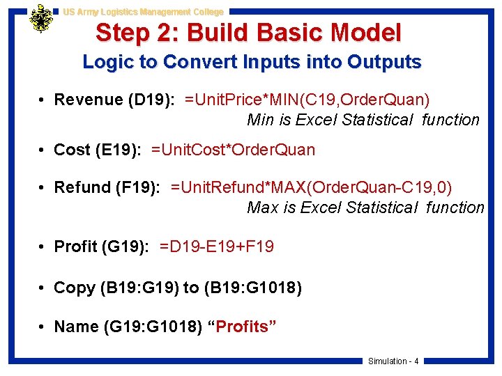
US Army Logistics Management College Step 2: Build Basic Model Logic to Convert Inputs into Outputs • Revenue (D 19): =Unit. Price*MIN(C 19, Order. Quan) Min is Excel Statistical function • Cost (E 19): =Unit. Cost*Order. Quan • Refund (F 19): =Unit. Refund*MAX(Order. Quan-C 19, 0) Max is Excel Statistical function • Profit (G 19): =D 19 -E 19+F 19 • Copy (B 19: G 19) to (B 19: G 1018) • Name (G 19: G 1018) “Profits” Simulation - 4

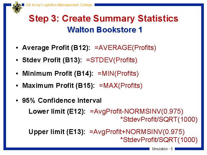
US Army Logistics Management College Step 3: Create Summary Statistics Walton Bookstore 1 • Average Profit (B 12): =AVERAGE(Profits) • Stdev Profit (B 13): =STDEV(Profits) • Minimum Profit (B 14): =MIN(Profits) • Maximum Profit (B 15): =MAX(Profits) • 95% Confidence Interval Lower limit (E 12): =Avg. Profit-NORMSINV(0. 975) *Stdev. Profit/SQRT(1000) Upper limit (E 13): =Avg. Profit+NORMSINV(0. 975) *Stdev. Profit/SQRT(1000) Simulation - 5

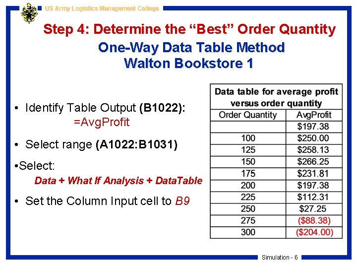
US Army Logistics Management College Step 4: Determine the “Best” Order Quantity One-Way Data Table Method Walton Bookstore 1 • Identify Table Output (B 1022): =Avg. Profit • Select range (A 1022: B 1031) • Select: Data + What If Analysis + Data. Table • Set the Column Input cell to B 9 Simulation - 6

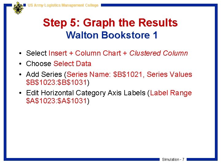
US Army Logistics Management College Step 5: Graph the Results Walton Bookstore 1 • Select Insert + Column Chart + Clustered Column • Choose Select Data • Add Series (Series Name: $B$1021, Series Values $B$1023: $B$1031) • Edit Horizontal Category Axis Labels (Label Range $A$1023: $A$1031) Simulation - 7

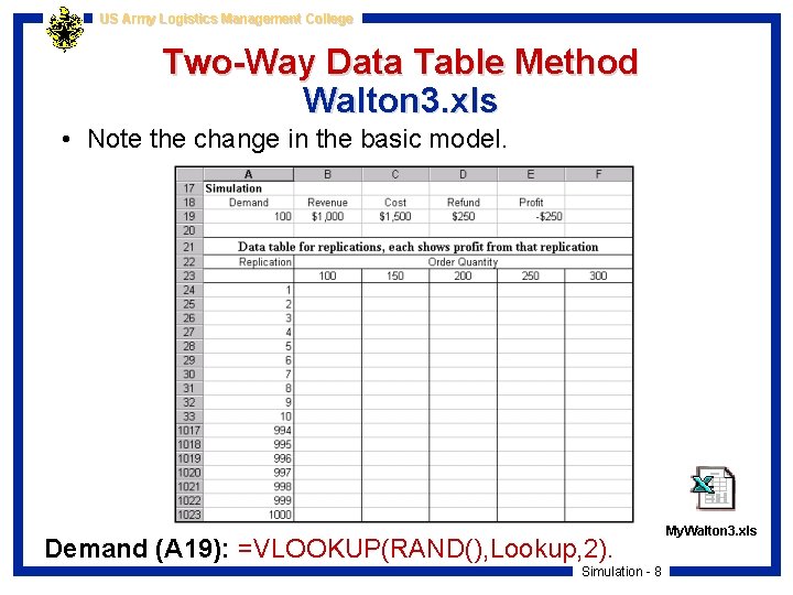
US Army Logistics Management College Two-Way Data Table Method Walton 3. xls • Note the change in the basic model. Demand (A 19): =VLOOKUP(RAND(), Lookup, 2). Simulation - 8 My. Walton 3. xls

US Army Logistics Management College Create the Two-Way Data Table Walton 3. xls • Identify Table Output (A 23): =Profit • Select range A 23: F 1023 for the Data Table • Select: Data + What If Analysis + Data. Table • For the Row input cell enter B 9 • For the Column Input cell enter G 23 or any other blank cell you choose. Simulation - 9

US Army Logistics Management College Part 2: Intro to Simulation Modeling with @Risk Simulation - 10

US Army Logistics Management College Walton Bookstore Revisited Walton 4. xls • Recall that Walton Bookstore buys calendars for $7. 50, sells them at a regular price of $10, and gets a refund for all calendars that cannot be sold. • The company does not know exactly how many calendars its customers will demand, but it does have historical data on demands for similar calendars in previous years. Walton wants to use these historical data to determine a reasonable probability distribution for next year’s demand for calendars. • Walton wants to use this probability distribution, together with @Risk, to simulate the profit for any particular order quantity. • Walton eventually wants to find the “best” order quantity. My. Walton 4. xls Simulation - 11

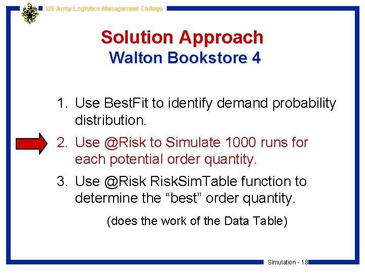
US Army Logistics Management College Solution Approach Walton Bookstore 4 1. Use Best. Fit to identify demand probability distribution. 2. Use @Risk to Simulate 1000 runs for each potential order quantity. 3. Use @Risk. Sim. Table function to determine the “best” order quantity. (does the work of the Data Table) Simulation - 12

US Army Logistics Management College Opening an Existing @Risk File 1. Open @Risk for Excel 2. Open the file: My. Walton 4. xls 3. Use File + Save As to save this file under a different name (such as Class My. Walton 4) Simulation - 13

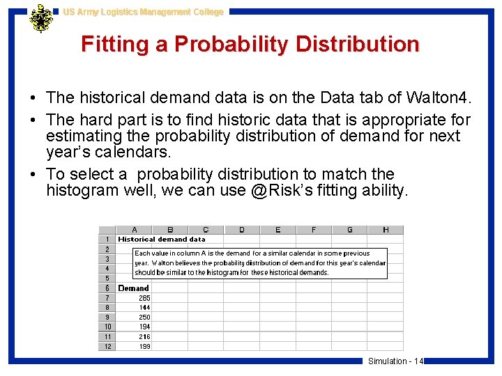
US Army Logistics Management College Fitting a Probability Distribution • The historical demand data is on the Data tab of Walton 4. • The hard part is to find historic data that is appropriate for estimating the probability distribution of demand for next year’s calendars. • To select a probability distribution to match the histogram well, we can use @Risk’s fitting ability. Simulation - 14

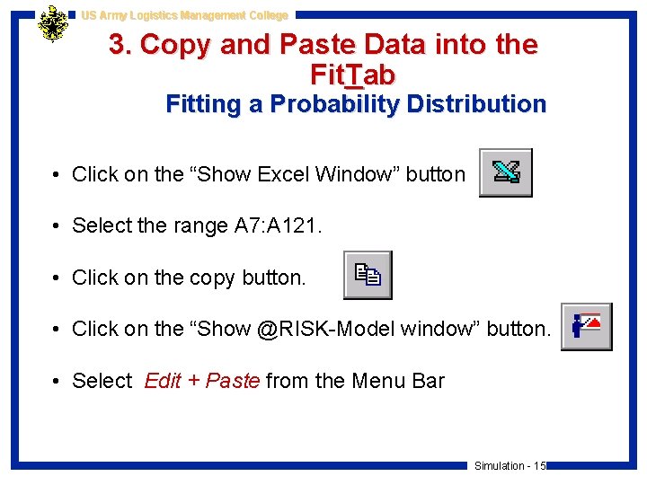
US Army Logistics Management College 3. Copy and Paste Data into the Fit. Tab Fitting a Probability Distribution • Click on the “Show Excel Window” button • Select the range A 7: A 121. • Click on the copy button. • Click on the “Show @RISK-Model window” button. • Select Edit + Paste from the Menu Bar Simulation - 15

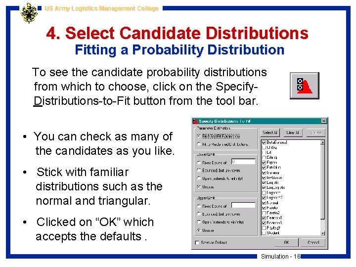
US Army Logistics Management College 4. Select Candidate Distributions Fitting a Probability Distribution To see the candidate probability distributions from which to choose, click on the Specify. Distributions-to-Fit button from the tool bar. • You can check as many of the candidates as you like. • Stick with familiar distributions such as the normal and triangular. • Clicked on “OK” which accepts the defaults. Simulation - 16

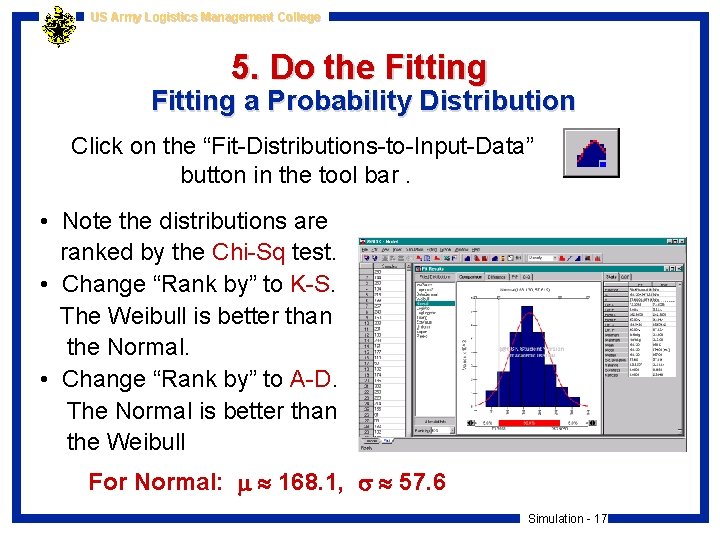
US Army Logistics Management College 5. Do the Fitting a Probability Distribution Click on the “Fit-Distributions-to-Input-Data” button in the tool bar. • Note the distributions are ranked by the Chi-Sq test. • Change “Rank by” to K-S. The Weibull is better than the Normal. • Change “Rank by” to A-D. The Normal is better than the Weibull For Normal: 168. 1, 57. 6 Simulation - 17

US Army Logistics Management College Solution Approach Walton Bookstore 4 1. Use Best. Fit to identify demand probability distribution. 2. Use @Risk to Simulate 1000 runs for each potential order quantity. 3. Use @Risk. Sim. Table function to determine the “best” order quantity. (does the work of the Data Table) Simulation - 18

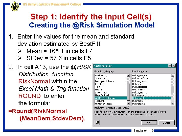
US Army Logistics Management College Step 1: Identify the Input Cell(s) Creating the @Risk Simulation Model 1. Enter the values for the mean and standard deviation estimated by Best. Fit! Ø Mean = 168. 1 in cells E 4 Ø St. Dev = 57. 6 in cells E 5. 2. In cell A 13, use the @RISK Distribution function Risk. Normal within the Excel Math & Trig function ROUND to enter the formula: =Round(Risk. Normal (Mean. Dem, Stdev. Dem). Simulation - 19

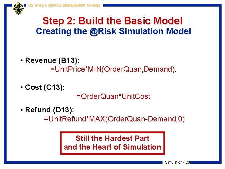
US Army Logistics Management College Step 2: Build the Basic Model Creating the @Risk Simulation Model • Revenue (B 13): =Unit. Price*MIN(Order. Quan, Demand). • Cost (C 13): =Order. Quan*Unit. Cost • Refund (D 13): =Unit. Refund*MAX(Order. Quan-Demand, 0) Still the Hardest Part and the Heart of Simulation - 20

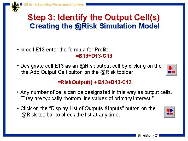
US Army Logistics Management College Step 3: Identify the Output Cell(s) Creating the @Risk Simulation Model • In cell E 13 enter the formula for Profit: =B 13+D 13 -C 13 • Designate cell E 13 as an @Risk output cell by clicking on the Add Output Cell button on the @Risk toolbar. =Risk. Output() + B 13+D 13 -C 13 • Any number of cells can be designated in this way as output cells. They are typically “bottom line values of primary interest. ” • Click on the “Display List of Outputs &Inputs” button on the @Risk toolbar to check the list at any time. Simulation - 21

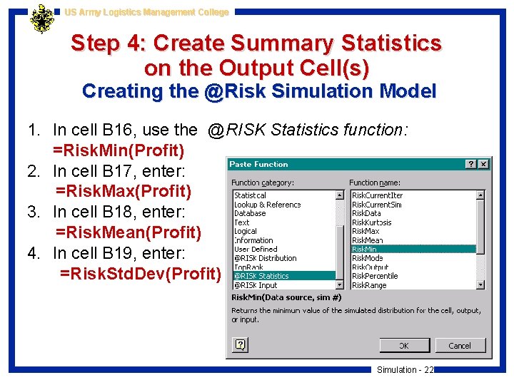
US Army Logistics Management College Step 4: Create Summary Statistics on the Output Cell(s) Creating the @Risk Simulation Model 1. In cell B 16, use the @RISK Statistics function: =Risk. Min(Profit) 2. In cell B 17, enter: =Risk. Max(Profit) 3. In cell B 18, enter: =Risk. Mean(Profit) 4. In cell B 19, enter: =Risk. Std. Dev(Profit) Simulation - 22

US Army Logistics Management College Step 5: Specify the Simulation Settings Creating the @Risk Simulation Model • Click on the “Simulations Settings” button. • Click on the “Iterations” tab in the Simulation Settings dialog box. Ø Set # Iterations to 1000. Ø Set # Simulations to 1. Ø Check Update Display. • Click on the “Sampling” tab in the Simulation Settings dialog box. Ø Ø Set Sampling Type to Latin Hypercube. Set Standard Recalc to Monte Carlo. Set Random Generator Seed to Choose Randomly. Set Collect Distribution Samples to All. Simulation - 23

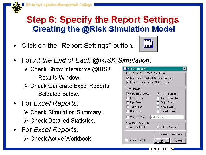
US Army Logistics Management College Step 6: Specify the Report Settings Creating the @Risk Simulation Model • Click on the “Report Settings” button. • For At the End of Each @RISK Simulation: Ø Check Show Interactive @RISK Results Window. Ø Check Generate Excel Reports Selected Below. • For Excel Reports: Ø Check Simulation Summary. Ø Check Detailed Statistics. • For Excel Reports: Ø Check Active Workbook. Simulation - 24

US Army Logistics Management College Step 6: Run the @Risk Simulation Creating the @Risk Simulation Model • To run the simulation, Click on the “Start Simulation” button. • In the @Risk Results window Ø To see Summary Statistics, use the “Summary Statistics Window” button. Ø To see Detailed Statistics, use the “Detailed Statistics Window” button. Simulation - 25

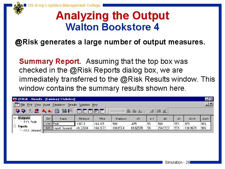
US Army Logistics Management College Analyzing the Output Walton Bookstore 4 @Risk generates a large number of output measures. Summary Report. Assuming that the top box was checked in the @Risk Reports dialog box, we are immediately transferred to the @Risk Results window. This window contains the summary results shown here. Simulation - 26

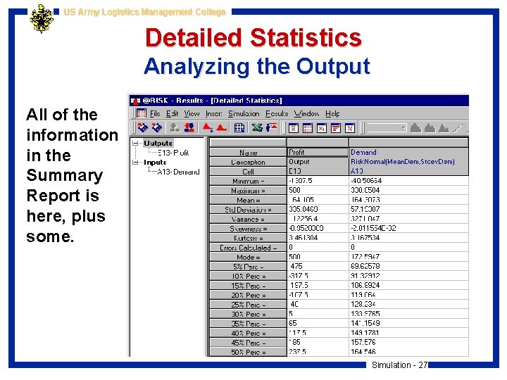
US Army Logistics Management College Detailed Statistics Analyzing the Output All of the information in the Summary Report is here, plus some. Simulation - 27

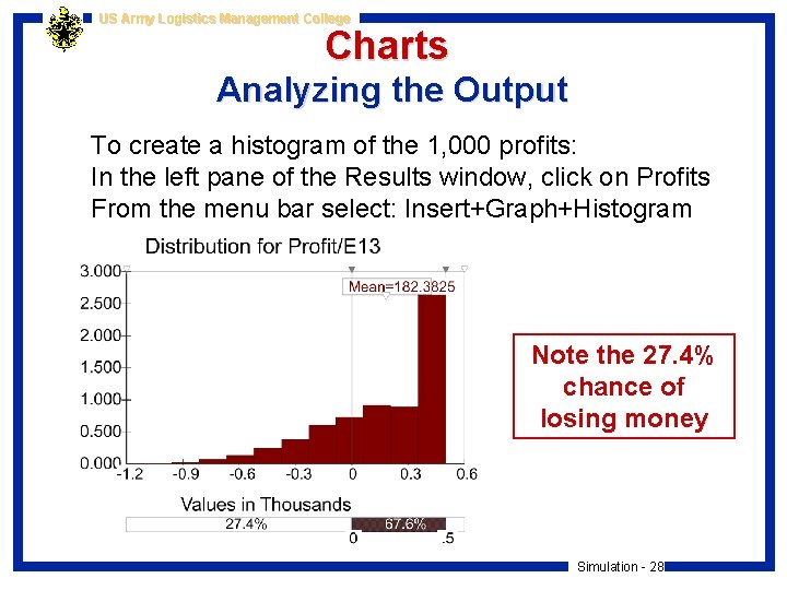
US Army Logistics Management College Charts Analyzing the Output To create a histogram of the 1, 000 profits: In the left pane of the Results window, click on Profits From the menu bar select: Insert+Graph+Histogram Note the 27. 4% chance of losing money Simulation - 28

US Army Logistics Management College Solution Approach Walton Bookstore 1. Use Best. Fit to identify demand probability distribution. 2. Use @Risk to Simulate 1000 runs for each potential order quantity. 3. Use @Risk. Sim. Table function to determine the “best” order quantity. (does the work of the Data Table) Simulation - 29

US Army Logistics Management College Using RISKSIMTABLE Walton Bookstore 5 • Walton’s ultimate goal is to choose an order quantity that provides a large average profit. • We could rerun the simulation model several times, each time with a different order quantity in the Order. Quan cell, and compare the results. • The RISKSIMTABLE function in @Risk enables us to obtain a fair comparison quickly and easily. • There are two modifications to the previous model. – We will create a list of order quantities to test. – Instead of entering a number in cell B 9 (the Order Quantity), we will use the @RISK function RISKSIMTABLE( ). My. Walton 5. xls Simulation - 30

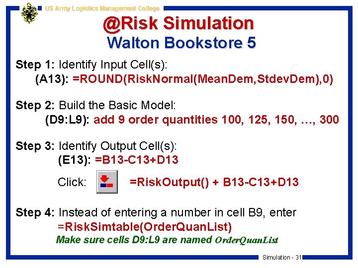
US Army Logistics Management College @Risk Simulation Walton Bookstore 5 Step 1: Identify Input Cell(s): (A 13): =ROUND(Risk. Normal(Mean. Dem, Stdev. Dem), 0) Step 2: Build the Basic Model: (D 9: L 9): add 9 order quantities 100, 125, 150, …, 300 Step 3: Identify Output Cell(s): (E 13): =B 13 -C 13+D 13 Click: =Risk. Output() + B 13 -C 13+D 13 Step 4: Instead of entering a number in cell B 9, enter =Risk. Simtable(Order. Quan. List) Make sure cells D 9: L 9 are named Order. Quan. List Simulation - 31

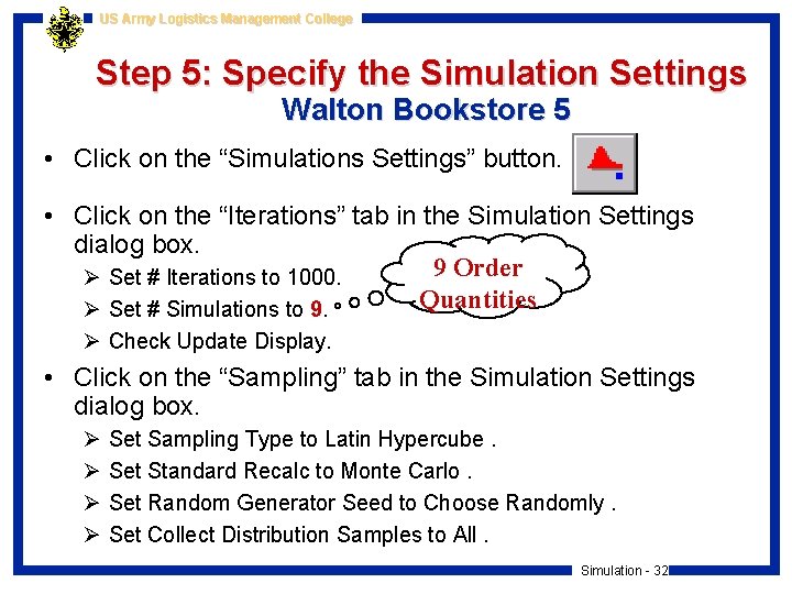
US Army Logistics Management College Step 5: Specify the Simulation Settings Walton Bookstore 5 • Click on the “Simulations Settings” button. • Click on the “Iterations” tab in the Simulation Settings dialog box. 9 Order Ø Set # Iterations to 1000. Quantities Ø Set # Simulations to 9. Ø Check Update Display. • Click on the “Sampling” tab in the Simulation Settings dialog box. Ø Ø Set Sampling Type to Latin Hypercube. Set Standard Recalc to Monte Carlo. Set Random Generator Seed to Choose Randomly. Set Collect Distribution Samples to All. Simulation - 32

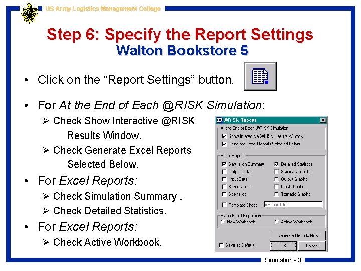
US Army Logistics Management College Step 6: Specify the Report Settings Walton Bookstore 5 • Click on the “Report Settings” button. • For At the End of Each @RISK Simulation: Ø Check Show Interactive @RISK Results Window. Ø Check Generate Excel Reports Selected Below. • For Excel Reports: Ø Check Simulation Summary. Ø Check Detailed Statistics. • For Excel Reports: Ø Check Active Workbook. Simulation - 33

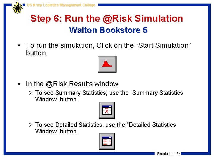
US Army Logistics Management College Step 6: Run the @Risk Simulation Walton Bookstore 5 • To run the simulation, Click on the “Start Simulation” button. • In the @Risk Results window Ø To see Summary Statistics, use the “Summary Statistics Window” button. Ø To see Detailed Statistics, use the “Detailed Statistics Window” button. Simulation - 34

US Army Logistics Management College Multiple Sources of Uncertainty Walton Bookstore 6 • As in previous examples, Walton needs to place an order for next year’s calendar. We continue to assume that the calendars will sell for $10 and customer demand for the calendars at this price is normally distributed with mean 168. 1 and standard deviation 57. 6. However, there are now two other sources of uncertainty. • First, the maximum number of calendars Walton’s supplier can supply is uncertain and is modeled with a triangular distribution. It’s parameters are 125, 250, and 200. Once Walton places an order, the supplier will charge $7. 50 per calendar if he can supply the entire Walton order. Otherwise, he will charge only $7. 25 per calendar. • Second, unsold calendars can no longer be returned to the supplier for a refund. Instead, Walton will put them on sale for $5 each after Feb 1. At that price, Walton believes the demand for leftover calendars is normally distributed with mean 50 and standard deviation 10. Any calendars still left over after March 1 will be thrown away. • Walton plans to order 200 calendars and wants to use simulation to analyze the resulting profit. Simulation - 35 My. Walton 6. xls

US Army Logistics Management College Part 3: @Risk Simulation Modeling An Example Simulation - 36

US Army Logistics Management College Drug Production Model with Uncertain Yields Trying to Meet an Order Due Date at Wozac • Wozac is a drug manufacturing company. It has recently accepted an order from its best customer for 8, 000 ounces of a new miracle drug, and wants to plan its production schedule to meet the customer’s promised delivery date of December 1, 2000. • There are three sources of uncertainty that make planning difficult. Simulation - 37

US Army Logistics Management College Sources of Uncertainty Wozac Drug Company • First, the drug must be produced in batches, and there is uncertainty about the time required to produce a batch, which could be anywhere from 5 to 11 days. This uncertainty is described by the discrete distribution of this table. Distribution of Days to Complete a Batch Days 5 6 7 8 9 10 11 Probability 0. 05 0. 10 0. 20 0. 30 0. 20 0. 10 0. 05 Simulation - 38

US Army Logistics Management College Sources of Uncertainty My Wozac Drugs. xls (Incomplete) Wozac Drug Company Continued Wozac Drugs. xls (Complete) • Second, the yield (usable quantity) from any batch is uncertain. Based on historical data, Wozac believes the yield can be modeled by a triangular distribution with parameters 600, 1000, 1100. • Third, all batches must go through a rigorous inspection once they are completed. The probability that a typical batch passes this inspection is only 0. 8. Therefore, the probability is 0. 2 that the batch fails inspection and none of it can be used to help fill the order. Wozac wants to use simulation to help decide how many days prior to the due date it should begin production. Simulation - 39

US Army Logistics Management College Building the Basic Model Wozac Drug Company • Batch Index: Limit of 25 by trial & error. Big enough. • Days (for this batch): (B 25: B 48): =IF(OR(F 24=“Yes”, F 24=“”), ” “, Risk. Discrete(Day, Probs)) The formula means: IF Enough? = Yes or is blank THEN Leave blank which acts as 0 ELSE Risk. Discrete(Day, Probs)) • Batch Yield: (C 25: C 48): =IF(OR(F 24=“Yes”, F 24=“”), ” “, Risk. Triang($D$19, $E$19, $F$19)) • Pass Inspection? (D 25: D 48): =IF(OR(F 24=“Yes”, F 24=“”), ” “, IF(Rand()<Pr. Pass, ”Yes”, ”No”)) Risk. Discrete & Risk. Triang are @Risk Distrib. functions Simulation - 40

US Army Logistics Management College Is the Order Filled? Col. E&F Building the Basic Model • Cum. Yield (cumulative usable product) (E 25: E 48): =IF(OR(F 24=“Yes”, F 24=“”), ” “, IF(D 25=“Yes”, C 25+E 24, E 24)) IF THEN ELSE Enough? = Yes or is blank Leave blank which acts as 0 IF this batch passed Then Add this batch to sum Else Use previous sum • Enough? (Is the order filled) (F 25: F 48): =IF(OR(F 24=“Yes”, F 24=“”), ” “, IF(E 25>=Amt. Reqd, ”Yes”, ”Not yet”)) IF THEN ELSE Enough? = Yes or is blank Leave blank which acts as 0 IF Cum. Yield>= cell B 5 Then Yes the order is filled Else No, we must do next row Simulation - 41

US Army Logistics Management College Run Summary Measures Building the Basic Model • Batches required (I 23): =COUNT(B 24: B 48) (count the cells that are not blank) • Days to complete (I 24): =SUM(B 24: B 48) (blanks count as 0) • Day to start (I 25): =Due. Date-Days. Reqd Ø Cell formatted for Date Ø Assumes 7 day production week I 23 & I 24 are @Risk Output cells, but we’ll handle that later Simulation - 42

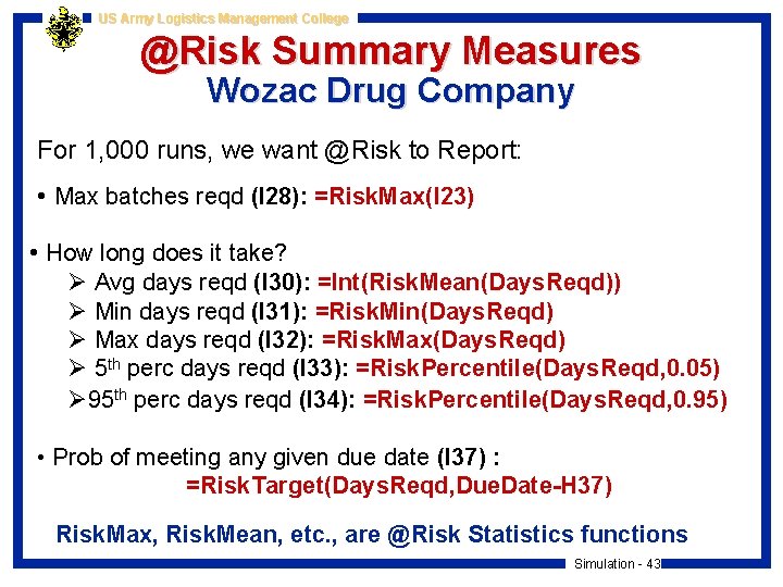
US Army Logistics Management College @Risk Summary Measures Wozac Drug Company For 1, 000 runs, we want @Risk to Report: • Max batches reqd (I 28): =Risk. Max(I 23) • How long does it take? Ø Avg days reqd (I 30): =Int(Risk. Mean(Days. Reqd)) Ø Min days reqd (I 31): =Risk. Min(Days. Reqd) Ø Max days reqd (I 32): =Risk. Max(Days. Reqd) Ø 5 th perc days reqd (I 33): =Risk. Percentile(Days. Reqd, 0. 05) Ø 95 th perc days reqd (I 34): =Risk. Percentile(Days. Reqd, 0. 95) • Prob of meeting any given due date (I 37) : =Risk. Target(Days. Reqd, Due. Date-H 37) Risk. Max, Risk. Mean, etc. , are @Risk Statistics functions Simulation - 43

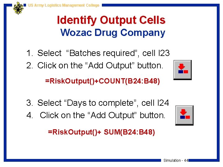
US Army Logistics Management College Identify Output Cells Wozac Drug Company 1. Select “Batches required”, cell I 23 2. Click on the “Add Output” button. =Risk. Output()+COUNT(B 24: B 48) 3. Select “Days to complete”, cell I 24 4. Click on the “Add Output” button. =Risk. Output()+ SUM(B 24: B 48) Simulation - 44

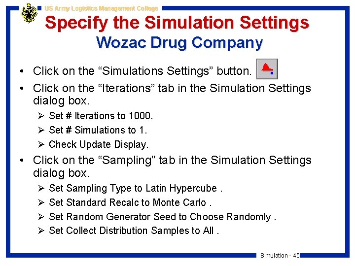
US Army Logistics Management College Specify the Simulation Settings Wozac Drug Company • Click on the “Simulations Settings” button. • Click on the “Iterations” tab in the Simulation Settings dialog box. Ø Set # Iterations to 1000. Ø Set # Simulations to 1. Ø Check Update Display. • Click on the “Sampling” tab in the Simulation Settings dialog box. Ø Ø Set Sampling Type to Latin Hypercube. Set Standard Recalc to Monte Carlo. Set Random Generator Seed to Choose Randomly. Set Collect Distribution Samples to All. Simulation - 45

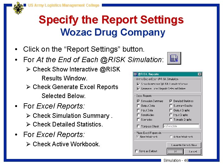
US Army Logistics Management College Specify the Report Settings Wozac Drug Company • Click on the “Report Settings” button. • For At the End of Each @RISK Simulation: Ø Check Show Interactive @RISK Results Window. Ø Check Generate Excel Reports Selected Below. • For Excel Reports: Ø Check Simulation Summary. Ø Check Detailed Statistics. • For Excel Reports: Ø Check Active Workbook. Simulation - 46

US Army Logistics Management College Run the @Risk Simulation Wozac Drug Company • To run the simulation, Click on the “Start Simulation” button. • In the @Risk Results window Ø To see Summary Statistics, use the “Summary Statistics Window” button. Ø To see Detailed Statistics, use the “Detailed Statistics Window” button. Simulation - 47

US Army Logistics Management College Part 4: Using Top. Rank with @Risk for Powerful Modeling Simulation - 48

US Army Logistics Management College New Product Development At SIMTEX • Sim. Tex, a pharmaceutical company, is in the early stages of developing a new drug called Biathnon. As with most new drugs, the future of Biathnon is highly uncertain. For example, its introduction into the market could be delayed, pending tests by the FDA. Also, its market could be diminished by a potential rival product from Sim. Tex’s competition. • Sim. Tex has identified a number of key inputs that will affect Biathnon’s future profitability: Simulation - 49

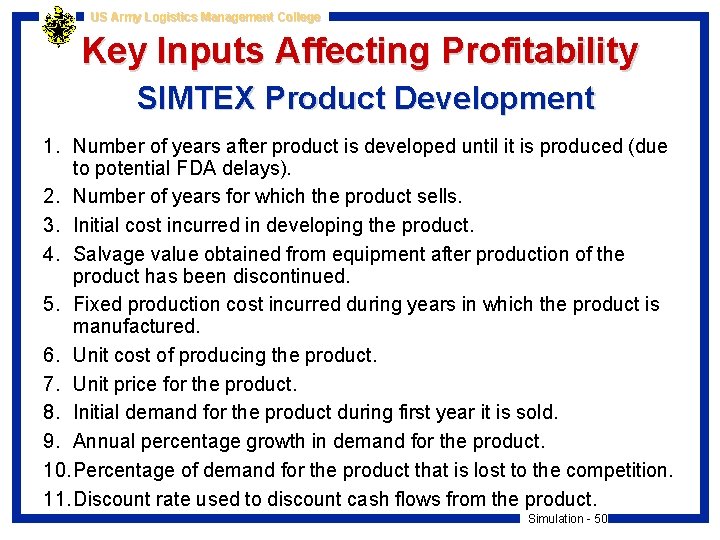
US Army Logistics Management College Key Inputs Affecting Profitability SIMTEX Product Development 1. Number of years after product is developed until it is produced (due to potential FDA delays). 2. Number of years for which the product sells. 3. Initial cost incurred in developing the product. 4. Salvage value obtained from equipment after production of the product has been discontinued. 5. Fixed production cost incurred during years in which the product is manufactured. 6. Unit cost of producing the product. 7. Unit price for the product. 8. Initial demand for the product during first year it is sold. 9. Annual percentage growth in demand for the product. 10. Percentage of demand for the product that is lost to the competition. 11. Discount rate used to discount cash flows from the product. Simulation - 50

US Army Logistics Management College Key Questions SIMTEX Product Development • How do changes in the inputs affect the key output, the Net Present Value of Biathnon over its lifetime? • Which inputs have a major affect on the Net Present Value of Biathnon over its lifetime? • How can Sim. Tex use Top. Rank and @Risk to analyze this problem? Sim. Tex 1. xls Simulation - 51

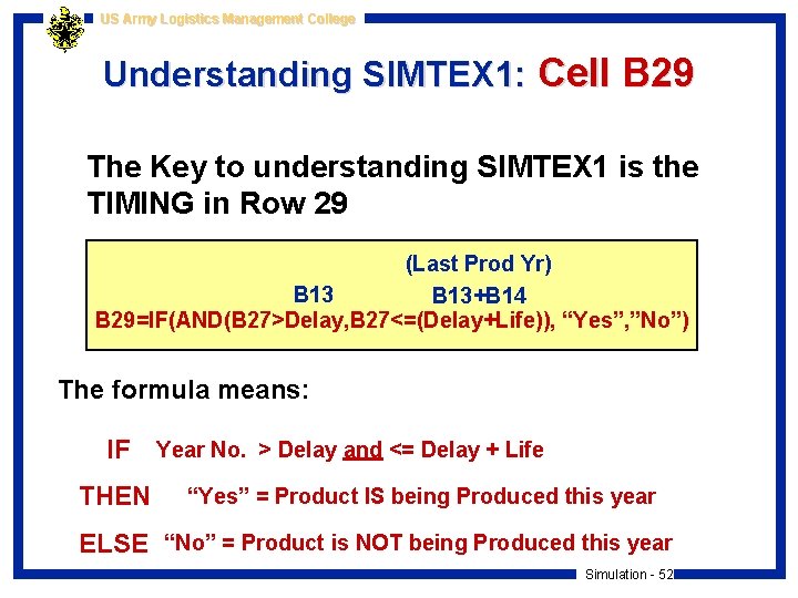
US Army Logistics Management College Understanding SIMTEX 1: Cell B 29 The Key to understanding SIMTEX 1 is the TIMING in Row 29 (Last Prod Yr) B 13+B 14 B 29=IF(AND(B 27>Delay, B 27<=(Delay+Life)), “Yes”, ”No”) The formula means: IF Year No. > Delay and <= Delay + Life THEN “Yes” = Product IS being Produced this year ELSE “No” = Product is NOT being Produced this year Simulation - 52

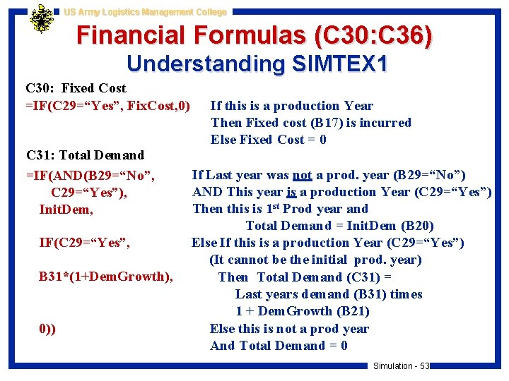
US Army Logistics Management College Financial Formulas (C 30: C 36) Understanding SIMTEX 1 C 30: Fixed Cost =IF(C 29=“Yes”, Fix. Cost, 0) C 31: Total Demand =IF(AND(B 29=“No”, C 29=“Yes”), Init. Dem, IF(C 29=“Yes”, B 31*(1+Dem. Growth), 0)) If this is a production Year Then Fixed cost (B 17) is incurred Else Fixed Cost = 0 If Last year was not a prod. year (B 29=“No”) AND This year is a production Year (C 29=“Yes”) Then this is 1 st Prod year and Total Demand = Init. Dem (B 20) Else If this is a production Year (C 29=“Yes”) (It cannot be the initial prod. year) Then Total Demand (C 31) = Last years demand (B 31) times 1 + Dem. Growth (B 21) Else this is not a prod year And Total Demand = 0 Simulation - 53

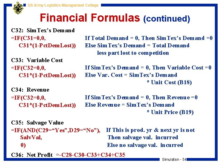
US Army Logistics Management College Financial Formulas (continued) C 32: Sim. Tex’s Demand =IF(C 31=0, 0, C 31*(1 -Pct. Dem. Lost)) C 33: Variable Cost =IF(C 32=0, 0, C 31*(1 -Pct. Dem. Lost)) C 34: Revenue =IF(C 32=0, 0, C 31*(1 -Pct. Dem. Lost)) If Total Demand = 0, Then Sim. Tex’s Demand =0 Else Sim. Tex’s Demand = Total Demand less part lost to competition If Sim. Tex’s Demand = 0, Then Variable Cost =0 Else Var. Cost = Sim. Tex’s Demand * Unit Cost (B 18) If Sim. Tex’s Demand = 0, Then Revenue =0 Else Revenue = Sim. Tex’s Demand * Unit Price (B 19) C 35: Salvage Value =IF(AND(C 29=“Yes”, D 29=“No”), If This is prod. yr & next yr is not Salv. Val, Then salvage val. incurred 0) Else no salvage val. incurred C 36: Net Profit =-C 28 -C 30 -C 33+C 34+C 35 Simulation - 54

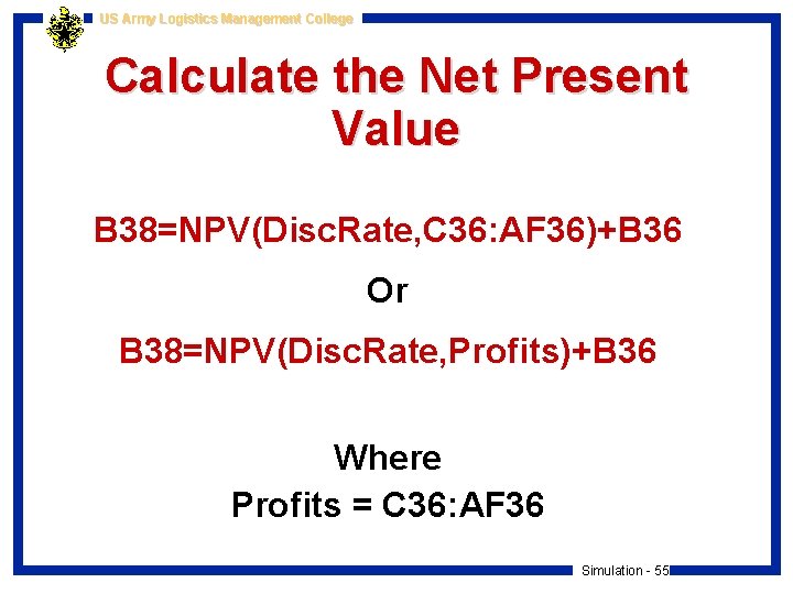
US Army Logistics Management College Calculate the Net Present Value B 38=NPV(Disc. Rate, C 36: AF 36)+B 36 Or B 38=NPV(Disc. Rate, Profits)+B 36 Where Profits = C 36: AF 36 Simulation - 55

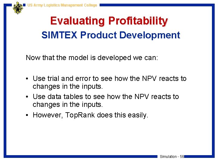
US Army Logistics Management College Evaluating Profitability SIMTEX Product Development Now that the model is developed we can: • Use trial and error to see how the NPV reacts to changes in the inputs. • Use data tables to see how the NPV reacts to changes in the inputs. • However, Top. Rank does this easily. Simulation - 56

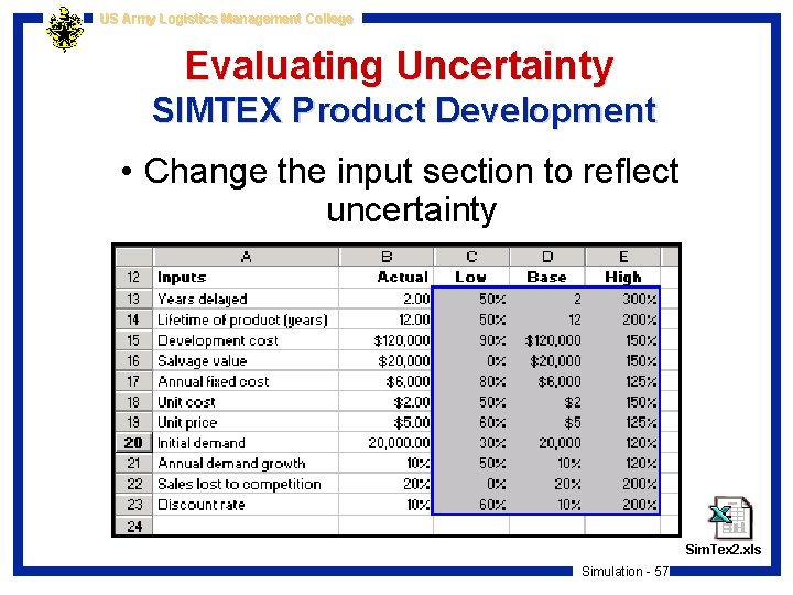
US Army Logistics Management College Evaluating Uncertainty SIMTEX Product Development • Change the input section to reflect uncertainty Sim. Tex 2. xls Simulation - 57

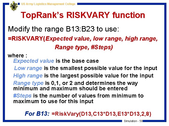
US Army Logistics Management College Top. Rank’s RISKVARY function Modify the range B 13: B 23 to use: =RISKVARY(Expected value, low range, high range, Range type, #Steps) where : Expected value is the base case Low range is the smallest possible value for the input High range is the largest possible value for the input Range type is 0, 1, or 2 and determines the way minimum and maximum should be entered #Steps is the number of values from minimum to maximum to use for this input For B 13: =Risk. Vary(D 13, C 13*D 13, E 13*D 13, 2, 8) Simulation - 58

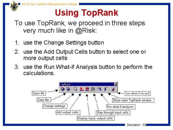
US Army Logistics Management College Using Top. Rank To use Top. Rank, we proceed in three steps very much like in @Risk: 1. use the Change Settings button 2. use the Add Output Cells button to select one or more output cells 3. use the Run What-if Analysis button to perform the calculations. Simulation - 59

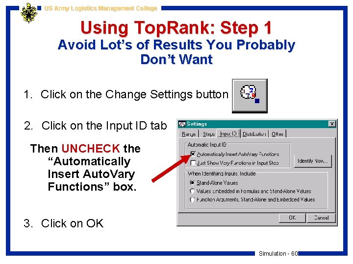
US Army Logistics Management College Using Top. Rank: Step 1 Avoid Lot’s of Results You Probably Don’t Want 1. Click on the Change Settings button 2. Click on the Input ID tab Then UNCHECK the “Automatically Insert Auto. Vary Functions” box. 3. Click on OK Simulation - 60

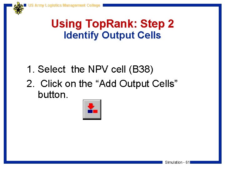
US Army Logistics Management College Using Top. Rank: Step 2 Identify Output Cells 1. Select the NPV cell (B 38) 2. Click on the “Add Output Cells” button. Simulation - 61

US Army Logistics Management College Using Top. Rank: Step 3 Run the Program Finally, run the analysis by clicking on the “Run What-if Analysis” button. Top. Rank then varies each input cell from its minimum to maximum, using the number of steps you specified and keeping the other inputs at their base levels, and keeps track of all the NPVs. Simulation - 62

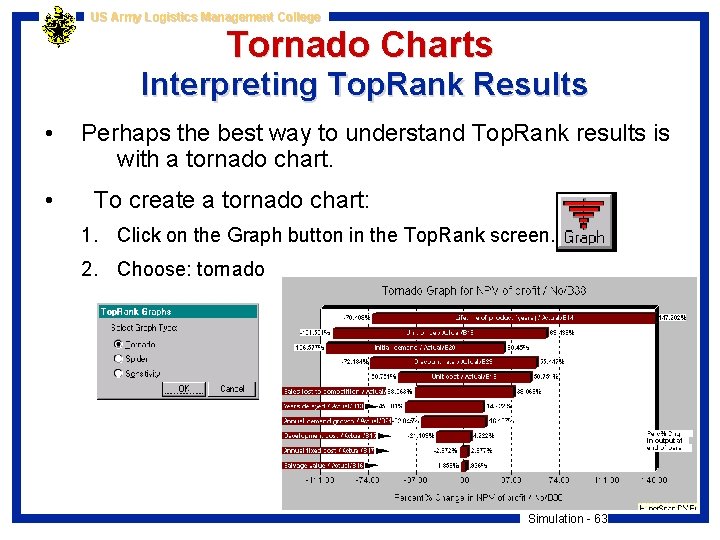
US Army Logistics Management College Tornado Charts Interpreting Top. Rank Results • • Perhaps the best way to understand Top. Rank results is with a tornado chart. To create a tornado chart: 1. Click on the Graph button in the Top. Rank screen. 2. Choose: tornado Simulation - 63

US Army Logistics Management College @Risk Simulation SIMTEX Product Development • We will run an @Risk simulation to estimate the distribution of NPV earned by Biathnon. • We will keep all inputs other than the five key inputs fixed at their base values. • We will use a triangular distribution for each of the random inputs: product lifetime, unit price, unit cost and initial demand • We will vary the discount rate systematically with the RISKSIMTABLE function. Simulation - 64

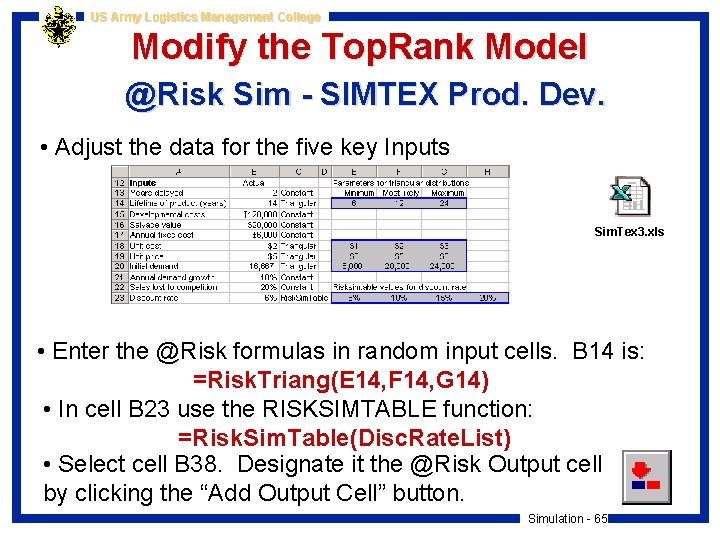
US Army Logistics Management College Modify the Top. Rank Model @Risk Sim - SIMTEX Prod. Dev. • Adjust the data for the five key Inputs Sim. Tex 3. xls • Enter the @Risk formulas in random input cells. B 14 is: =Risk. Triang(E 14, F 14, G 14) • In cell B 23 use the RISKSIMTABLE function: =Risk. Sim. Table(Disc. Rate. List) • Select cell B 38. Designate it the @Risk Output cell by clicking the “Add Output Cell” button. Simulation - 65

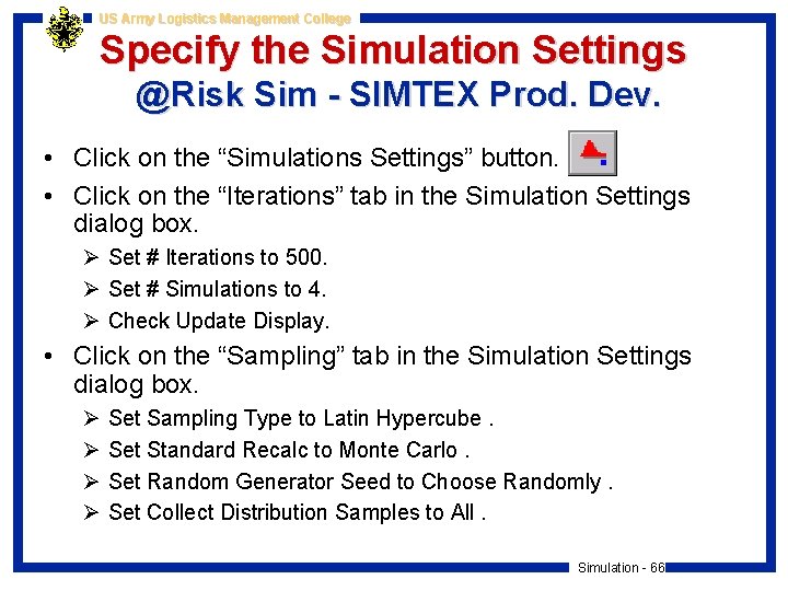
US Army Logistics Management College Specify the Simulation Settings @Risk Sim - SIMTEX Prod. Dev. • Click on the “Simulations Settings” button. • Click on the “Iterations” tab in the Simulation Settings dialog box. Ø Set # Iterations to 500. Ø Set # Simulations to 4. Ø Check Update Display. • Click on the “Sampling” tab in the Simulation Settings dialog box. Ø Ø Set Sampling Type to Latin Hypercube. Set Standard Recalc to Monte Carlo. Set Random Generator Seed to Choose Randomly. Set Collect Distribution Samples to All. Simulation - 66

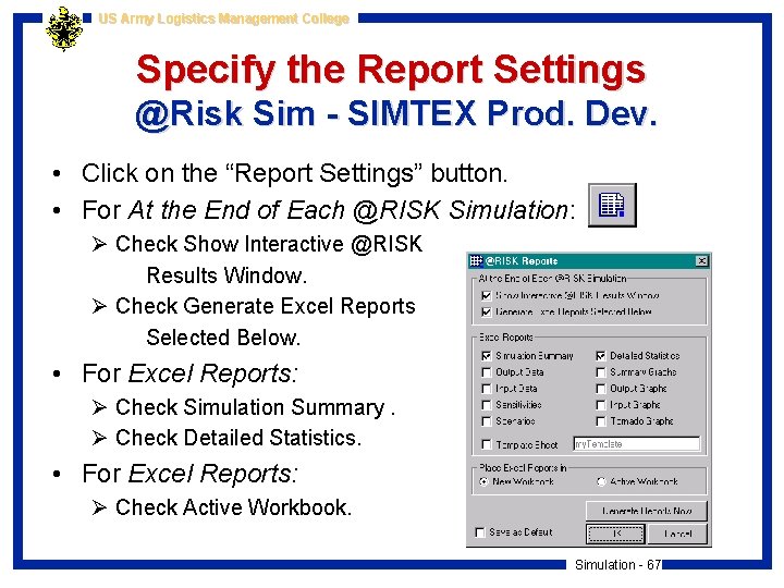
US Army Logistics Management College Specify the Report Settings @Risk Sim - SIMTEX Prod. Dev. • Click on the “Report Settings” button. • For At the End of Each @RISK Simulation: Ø Check Show Interactive @RISK Results Window. Ø Check Generate Excel Reports Selected Below. • For Excel Reports: Ø Check Simulation Summary. Ø Check Detailed Statistics. • For Excel Reports: Ø Check Active Workbook. Simulation - 67

US Army Logistics Management College Run the @Risk Simulation SIMTEX Product Development • To run the simulation, Click on the “Start Simulation” button. • In the @Risk Results window Ø To see Summary Statistics, use the “Summary Statistics Window” button. Ø To see Detailed Statistics, use the “Detailed Statistics Window” button. Simulation - 68

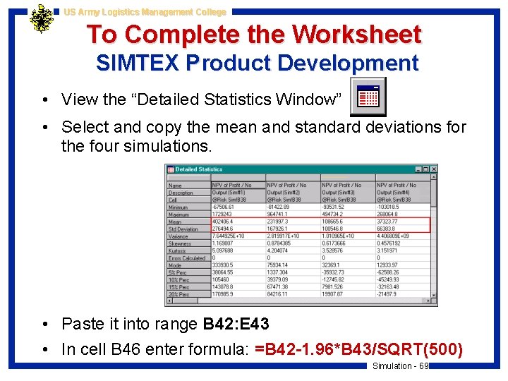
US Army Logistics Management College To Complete the Worksheet SIMTEX Product Development • View the “Detailed Statistics Window” • Select and copy the mean and standard deviations for the four simulations. • Paste it into range B 42: E 43 • In cell B 46 enter formula: =B 42 -1. 96*B 43/SQRT(500) Simulation - 69