US Army Logistics Management College Math Programming Intro




- Slides: 99

US Army Logistics Management College Math Programming Intro to Optimization Modeling, Linear Programming Models, and Network Models Math Programming - 1

US Army Logistics Management College Introduction to LP Modeling Producing Frames at the Monet Company Math Programming - 2

US Army Logistics Management College Background Information Producing Frames at the Monet Company • The Monet Company produces four type of picture frames that differ with respect to size, shape, materials used, labor required and selling price • During the coming week Monet can purchase up to 4000 hours of skilled labor, 6000 ounces of metal, and 10, 000 ounces of glass • Market constraints limit sales to no more than 1000 type 1 frames, 2000 type 2, frames, 500 type 3 frames, and 1000 type 4 frames • The company wants to maximize its weekly profit Math Programming - 3

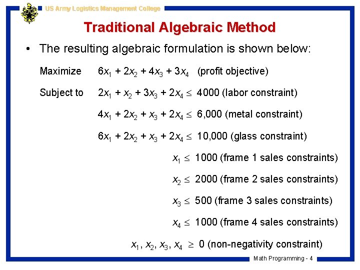
US Army Logistics Management College Traditional Algebraic Method • The resulting algebraic formulation is shown below: Maximize 6 x 1 + 2 x 2 + 4 x 3 + 3 x 4 (profit objective) Subject to 2 x 1 + x 2 + 3 x 3 + 2 x 4 4000 (labor constraint) 4 x 1 + 2 x 2 + x 3 + 2 x 4 6, 000 (metal constraint) 6 x 1 + 2 x 2 + x 3 + 2 x 4 10, 000 (glass constraint) x 1 1000 (frame 1 sales constraints) x 2 2000 (frame 2 sales constraints) x 3 500 (frame 3 sales constraints) x 4 1000 (frame 4 sales constraints) x 1, x 2, x 3, x 4 0 (non-negativity constraint) Math Programming - 4

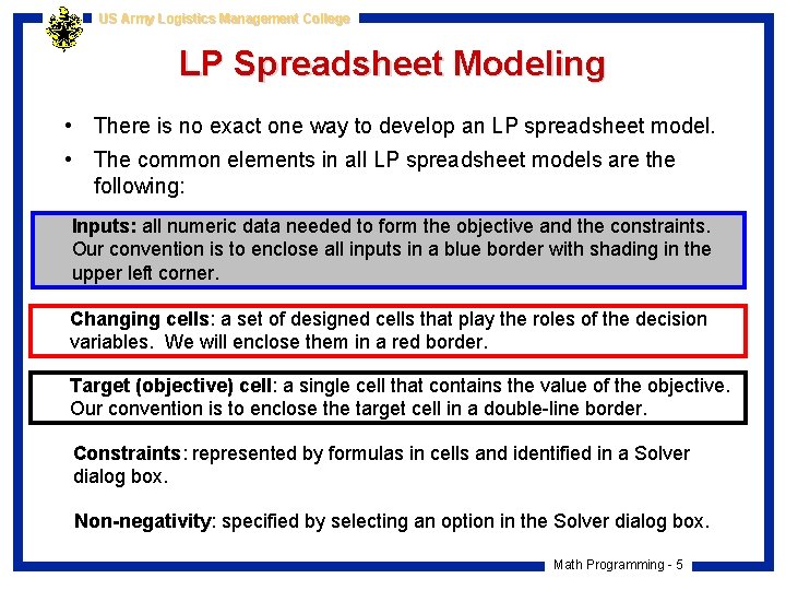
US Army Logistics Management College LP Spreadsheet Modeling • There is no exact one way to develop an LP spreadsheet model. • The common elements in all LP spreadsheet models are the following: Inputs: all numeric data needed to form the objective and the constraints. Our convention is to enclose all inputs in a blue border with shading in the upper left corner. Changing cells: a set of designed cells that play the roles of the decision variables. We will enclose them in a red border. Target (objective) cell: a single cell that contains the value of the objective. Our convention is to enclose the target cell in a double-line border. Constraints: represented by formulas in cells and identified in a Solver dialog box. Non-negativity: specified by selecting an option in the Solver dialog box. Math Programming - 5

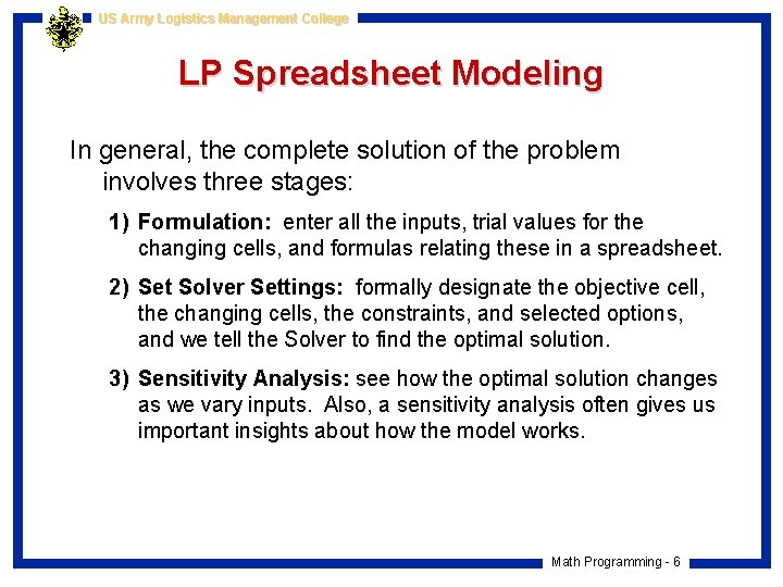
US Army Logistics Management College LP Spreadsheet Modeling In general, the complete solution of the problem involves three stages: 1) Formulation: enter all the inputs, trial values for the changing cells, and formulas relating these in a spreadsheet. 2) Set Solver Settings: formally designate the objective cell, the changing cells, the constraints, and selected options, and we tell the Solver to find the optimal solution. 3) Sensitivity Analysis: see how the optimal solution changes as we vary inputs. Also, a sensitivity analysis often gives us important insights about how the model works. Math Programming - 6

US Army Logistics Management College Model Formulation Producing Frames at the Monet Company • The first stage is to setup the spreadsheet – Inputs: Enter numeric inputs in the shaded ranges. – Production levels: Enter trial values in the range named Produced – Resources used: Enter formulas for labor, metal, & glass =SUMPRODUCT (B 9: E 9, Produced) in cell B 21 and copy – Revenue: enter the formula =B 12*B 16 in cell B 27 and copy – Cost: enter the formula =$B 4*B$16*B 9 in cell B 29 and copy – Profit: enter the formula =B 27 -SUM(B 29: B 31) in cell B 32 and copy – Calculate total revenues, costs, and profit in column F Math Programming - 7

US Army Logistics Management College Model Formulation Enter Trial Values • Why should we input trial values in the changing cells? – Verification: entering different sets of values in the changing cells allow us to confirm that the formulas are working correctly – Trial values help us to understand the model – Good estimates of trial values can help find the solution in a shorter number of iterations • For example, it is tempting to guess that the frame types with the highest profit margins should be produced to the greatest extent possible • Does this guarantee that this solution is the best possible product mix? Unfortunately, it does not! Math Programming - 8

US Army Logistics Management College Set Solver Settings Producing Frames at the Monet Company • The second stage is to estimate an initial solution and specify the Solver settings (Solver is on Data Ribbon) • To enter information, type cell references or point, click and drag – Objective: Select Tot. Profit cell as the target cell (set to Maximize) – Changing cells: Select the Produced range, (numbers of frames produced) – Constraints: Click on the Add button to add the following constraints: » Used<=Available (can’t use more than available resources) » Produced<=Max. Sales (produce no more than demand of each product) Math Programming - 9

US Army Logistics Management College Set Solver Settings Producing Frames at the Monet Company • Setting Solver Options – Non-negativity: Make all changing cells non-negative – Linear model: Uses a Simplex based algorithm to solve the model » Changing cells cannot be multiplied by other changing cells used as a Solver input » Changing cells cannot be raised to a power or be a part of other non-linear EXCEL functions » The changing cell cannot be a part of the right hand side of a constraint in the Solver constraint box » If a model is not linear and assume linear model is checked, an error message will be displayed » If assume linear model is NOT checked, a non-linear solution method will be used Math Programming - 10

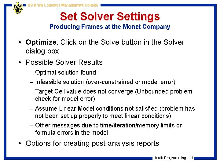
US Army Logistics Management College Set Solver Settings Producing Frames at the Monet Company • Optimize: Click on the Solve button in the Solver dialog box • Possible Solver Results – Optimal solution found – Infeasible solution (over-constrained or model error) – Target Cell value does not converge (Unbounded problem – check for model error) – Assume Linear Model conditions not satisfied (problem has not been set up properly to meet linear conditions) – Other messages due to time/iteration/memory limits or formula errors in the model • Options for creating post-analysis reports Math Programming - 11

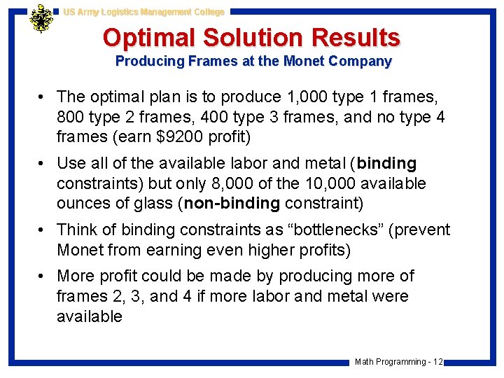
US Army Logistics Management College Optimal Solution Results Producing Frames at the Monet Company • The optimal plan is to produce 1, 000 type 1 frames, 800 type 2 frames, 400 type 3 frames, and no type 4 frames (earn $9200 profit) • Use all of the available labor and metal (binding constraints) but only 8, 000 of the 10, 000 available ounces of glass (non-binding constraint) • Think of binding constraints as “bottlenecks” (prevent Monet from earning even higher profits) • More profit could be made by producing more of frames 2, 3, and 4 if more labor and metal were available Math Programming - 12

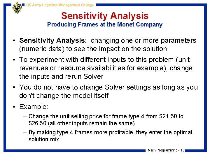
US Army Logistics Management College Sensitivity Analysis Producing Frames at the Monet Company • Sensitivity Analysis: changing one or more parameters (numeric data) to see the impact on the solution • To experiment with different inputs to this problem (unit revenues or resource availabilities for example), change the inputs and rerun Solver • You do not have to change Solver settings as long as you don’t change the model itself • Example: – Change the unit selling price for frame type 4 from $21. 50 to $26. 50 (all other inputs remain the same) – By making type 4 frames more profitable, they enter the optimal solution mix Math Programming - 13

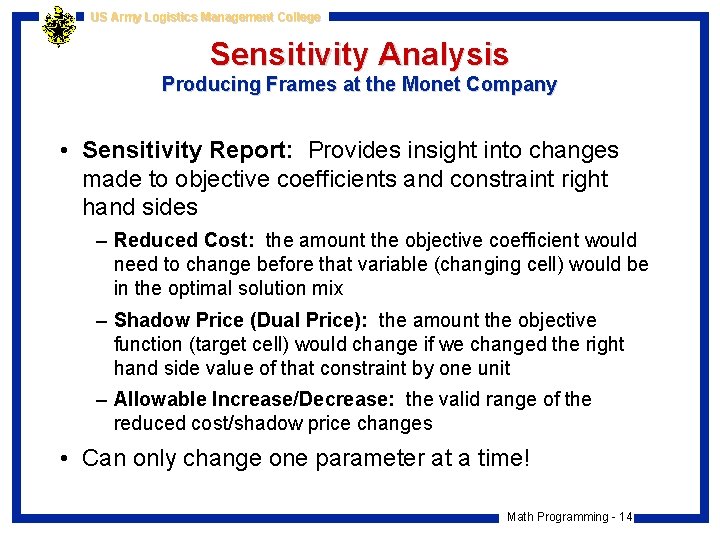
US Army Logistics Management College Sensitivity Analysis Producing Frames at the Monet Company • Sensitivity Report: Provides insight into changes made to objective coefficients and constraint right hand sides – Reduced Cost: the amount the objective coefficient would need to change before that variable (changing cell) would be in the optimal solution mix – Shadow Price (Dual Price): the amount the objective function (target cell) would change if we changed the right hand side value of that constraint by one unit – Allowable Increase/Decrease: the valid range of the reduced cost/shadow price changes • Can only change one parameter at a time! Math Programming - 14

US Army Logistics Management College Sensitivity Analysis and the Solver Table Add-In • Solver Table Add-In allows analysis of one or two parameter changes over a range specified by the modeler • Similar to data table, except will optimize each cell entry in the table • Provides for more flexibility and visual display of sensitivity analysis than sensitivity analysis report Math Programming - 15

US Army Logistics Management College Solver Table Add-In Producing Frames at the Monet Company • Setting up a Solver Table: – Select Data/Solver. Table menu item – Select Oneway or Twoway table in the first dialog box – Select input cell(s) (parameter you want to change) – Select values for input cells (either min, max, increment or list specific values) – Select output cell(s) (typically target cell and others) – Select location of table (specify upper left corner) • Click OK and Solver solves a separate optimization problem for each of the cells in the table and reports the requested outputs Math Programming - 16

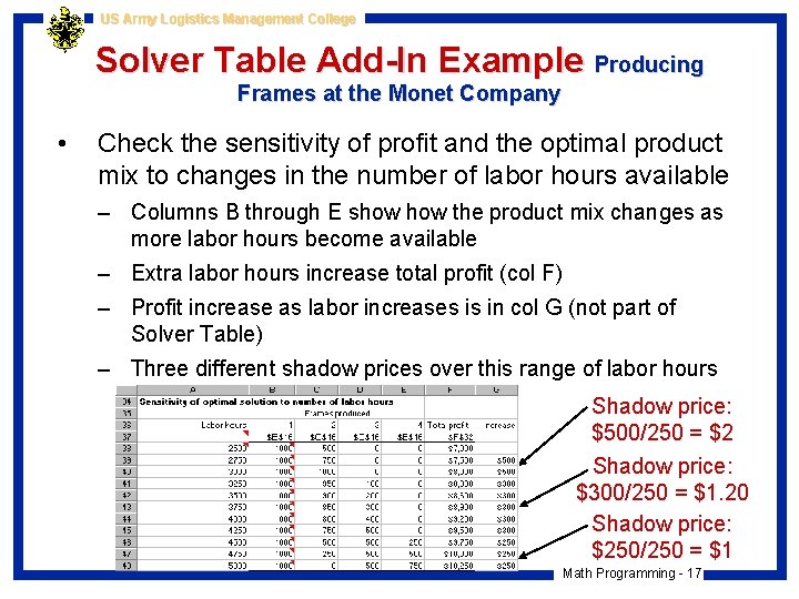
US Army Logistics Management College Solver Table Add-In Example Producing Frames at the Monet Company • Check the sensitivity of profit and the optimal product mix to changes in the number of labor hours available – Columns B through E show the product mix changes as more labor hours become available – Extra labor hours increase total profit (col F) – Profit increase as labor increases is in col G (not part of Solver Table) – Three different shadow prices over this range of labor hours Shadow price: $500/250 = $2 Shadow price: $300/250 = $1. 20 Shadow price: $250/250 = $1 Math Programming - 17

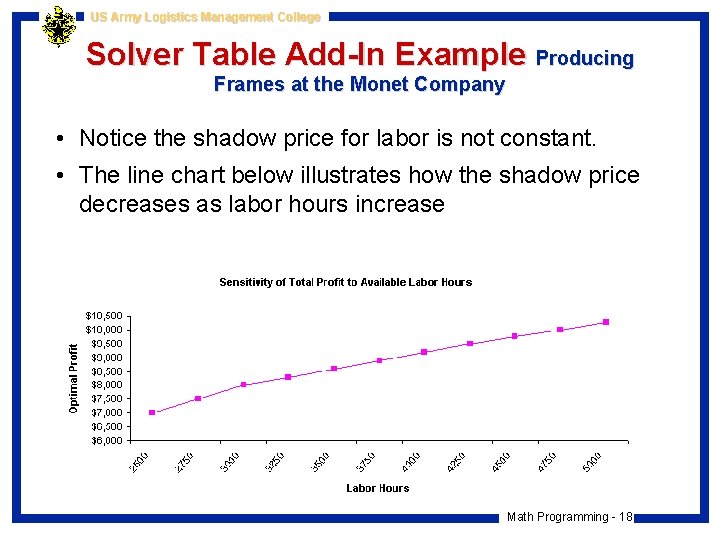
US Army Logistics Management College Solver Table Add-In Example Producing Frames at the Monet Company • Notice the shadow price for labor is not constant. • The line chart below illustrates how the shadow price decreases as labor hours increase Math Programming - 18

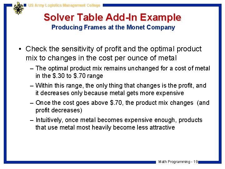
US Army Logistics Management College Solver Table Add-In Example Producing Frames at the Monet Company • Check the sensitivity of profit and the optimal product mix to changes in the cost per ounce of metal – The optimal product mix remains unchanged for a cost of metal in the $. 30 to $. 70 range – Within this range, the only thing that changes is the profit, and it decreases only because metal gets more expensive – Once the cost goes above $. 70, the product mix changes (and profit decreases) – Intuitively, once metal becomes expensive enough, products that use metal most heavily become less attractive Math Programming - 19

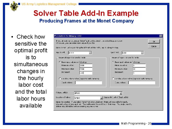
US Army Logistics Management College Solver Table Add-In Example Producing Frames at the Monet Company • Check how sensitive the optimal profit is to simultaneous changes in the hourly labor cost and the total labor hours available Math Programming - 20

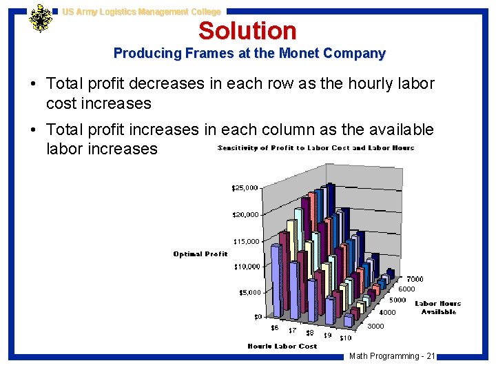
US Army Logistics Management College Solution Producing Frames at the Monet Company • Total profit decreases in each row as the hourly labor cost increases • Total profit increases in each column as the available labor increases Math Programming - 21

US Army Logistics Management College Aggregate Planning Models Worker and Production Planning at Sure. Step Math Programming - 22

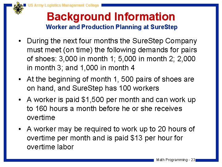
US Army Logistics Management College Background Information Worker and Production Planning at Sure. Step • During the next four months the Sure. Step Company must meet (on time) the following demands for pairs of shoes: 3, 000 in month 1; 5, 000 in month 2; 2, 000 in month 3; and 1, 000 in month 4 • At the beginning of month 1, 500 pairs of shoes are on hand, and Sure. Step has 100 workers • A worker is paid $1, 500 per month and can work up to 160 hours a month before he or she receives overtime • A worker may be required to work up to 20 hours of overtime per month and is paid $13 per hour for overtime labor Math Programming - 23

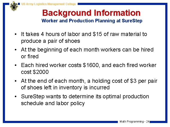
US Army Logistics Management College Background Information Worker and Production Planning at Sure. Step • It takes 4 hours of labor and $15 of raw material to produce a pair of shoes • At the beginning of each month workers can be hired or fired • Each hired worker costs $1600, and each fired worker cost $2000 • At the end of each month, a holding cost of $3 per pair of shoes left in inventory is incurred • Sure. Step wants to determine its optimal production schedule and labor policy Math Programming - 24

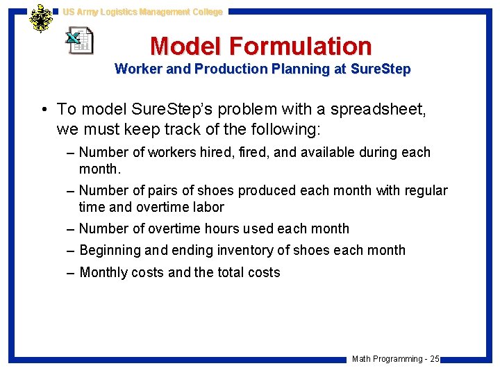
US Army Logistics Management College Model Formulation Worker and Production Planning at Sure. Step • To model Sure. Step’s problem with a spreadsheet, we must keep track of the following: – Number of workers hired, fired, and available during each month. – Number of pairs of shoes produced each month with regular time and overtime labor – Number of overtime hours used each month – Beginning and ending inventory of shoes each month – Monthly costs and the total costs Math Programming - 25

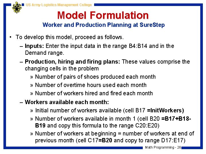
US Army Logistics Management College Model Formulation Worker and Production Planning at Sure. Step • To develop this model, proceed as follows. – Inputs: Enter the input data in the range B 4: B 14 and in the Demand range. – Production, hiring and firing plans: These values comprise the changing cells in the problem » Number of pairs of shoes produced each month » Number of overtime hours used each month » Number of workers hired and fired each month – Workers available each month: » Initial number of workers available (cell B 17 =Init. Workers) » Number of workers available in month 1 (cell B 20 =B 17+B 18 B 19 and copy this formula to the range C 20: E 20) » Number of workers at beginning = number of workers at end of previous month (cell C 17=B 20 and copy to range D 17: E 17) Math Programming - 26

US Army Logistics Management College Model Formulation Worker and Production Planning at Sure. Step – Overtime capacity: Each available worker can work up to 20 hours of overtime in a month (cell B 25 =Max. OTHrs*B 20 and copy it to the range C 25: E 25) – Production capacity: » Each worker can work 160 regular-time hours per month (cell B 22 =Std. RTHrs*B 20 and copy it to the range C 22: E 22) » Sum the total monthly production hours available (cell B 27 =SUM(B 23: B 24) and copy it to the range C 27: E 27) » Calculate the production capacity using the labor hours for shoes (cell B 32 =B 27/Hrs. Per. Pair and copy it to the range C 32: E 32) Math Programming - 27

US Army Logistics Management College Model Formulation Worker and Production Planning at Sure. Step – Monthly inventory: » Inventory after production in month 1 (cell B 34 =Init. Inv+B 30) » For other months, inventory after production is the previous month’s ending inventory plus this month’s production (cell C 34 =B 37+C 30 and copy it to the range D 34: E 34) » Ending inventory is inventory after production less demand (cell B 37 =B 34 -B 36 and copy it to the range C 37: E 37) – Monthly costs: Calculate the various costs shown in rows 40 through 45 (cell B 40 =Unit. Hire. Cost*B 18, cell B 41 =Unit. Fire. Cost*B 19, cell B 42 =RTWage. Rate*B 20, cell B 43 =OTWage. Rate*B 23, cell B 44 =Unit. Mat. Cost*B 30, cell B 45 =Unit. Hold. Cost*B 37 and copy B 40: B 45 to the range C 40: E 45) Math Programming - 28

US Army Logistics Management College Set Solver Settings Worker and Production Planning at Sure. Step • Invoking the Solver – Objective: Target cell is minimize Tot. Cost – Changing cells: Hired, Fired, Production, and OTHrs – Overtime constraints: OTHrs <= OTAvailable – Production capacity constraint: Production<=Prod. Cap – Demand constraint: On. Hand>=Demand – Integer constraints: Constrain the number hired and fired to be integers – Specify non-negativity, assume linear, and optimize Math Programming - 29

US Army Logistics Management College Optimal Solution Worker and Production Planning at Sure. Step • The company produces slightly over 3700 pairs of shoes during each of the first 2 months, 200 pairs in month 3, and 1000 in month 4 • Sure. Step should never hire any workers • Fire 6 workers in month 1, 1 worker in month 2, and 43 workers in month 3 • Eighty hours of overtime are used (only in month 2) • Minimum total cost of $692, 820 Math Programming - 30

US Army Logistics Management College Optimal Solution – Integer Considerations Worker and Production Planning at Sure. Step • It is important to ensure that the number of workers hired and fired each month is an integer, given the small number of workers involved • The number of pairs of shoes produced each month does not have to be solved as an integer (due to the large quantity) • To ensure that Solver finds the optimal solution in a problem where some or all of the changing cells must be integers, go into Options, then to Integer Options, and set the tolerance to 0 • If the tolerance is set to a value other than 0, Solver might stop when it finds a solution that is close to optimal Math Programming - 31

US Army Logistics Management College Model with Backlogging Allowed Worker and Production Planning at Sure. Step • In many situations backlogging is allowed, that is, customer demand, can be met later than it occurs. • We’ll modify this example to include the option of backlogged demand. • We assume that at the end of each month a cost of $20 is incurred for each unit of demand that remains unsatisfied at the end of the month. • This is easily modeled by allowing a month’s ending inventory to be negative. The last month, month 4, should be nonnegative. This also ensures that all demand will eventually be met by the end of the fourmonth horizon. Math Programming - 32

US Army Logistics Management College Model with Backlogging Allowed Worker and Production Planning at Sure. Step • Model the previous problem to allow backlogging (demand does not have to be met in the same month, but can be met later at some additional cost) • To allow backlogging, modify the monthly cost computations to incorporate the costs due to shortages • Two possible modeling approaches: – The first is the more “natural”, but it results in a nonlinear model – The second is more complicated, but allows for a linear model Math Programming - 33

US Army Logistics Management College Backlogging – Nonlinear Approach Worker and Production Planning at Sure. Step • Enter the per unit monthly shortage cost in the Unit. Short. Cost cell • Remove <= signs for months 1 -3 • Adjust holding and shortage cost formulas in rows 46 and 47: – For holding costs: cell B 46 =IF(B 38>0, Unit. Hold. Cost*B 38, 0) and copy across – For shortage costs: cell B 47 =IF(B 38<0, -Unit. Short. Cost*B 38, 0) and copy across • Adjust Solver Settings so that inventory on hand meets or exceeds demand for month 4 only Math Programming - 34

US Army Logistics Management College Backlogging – Nonlinear Approach Worker and Production Planning at Sure. Step • Use of IF functions make the objective function nonlinear (Do not check Assume Linear option) • Problem with nonlinear approach: solution found not guaranteed to be global optimal • Tips on finding good nonlinear solutions: – Start with initial trial values for your adjustable cells that seem like a good solution – Vary your initial trial values and see if the solution changes – Read the help screen for the Solver Options dialog box to understand settings associated with nonlinear problems Math Programming - 35

US Army Logistics Management College Backlogging –Linear Approach Worker and Production Planning at Sure. Step • Enter per unit monthly shortage cost in the Unit. Short. Cost cell • Create rows for excess, shortage, and net inventory (B 39: E 41): – The excess range in row 39 contains the amounts left in inventory – The shortage range in row 40 contains unmet demand (backlog) – The net Inventory is excess inventory – shortage inventory Math Programming - 36

US Army Logistics Management College Backlogging –Linear Approach Worker and Production Planning at Sure. Step • Note that if we force net inventory to equal the ending inventory (which equals inventory after production less demand), then one of three conditions occur: – Excess inventory > 0, shortage inventory = 0 (surplus) – Excess inventory = 0, shortage inventory > 0 (shortage) – Excess inventory = 0, shortage inventory = 0 (balanced) • Adjust holding and shortage cost formulas in rows 51 and 52 – – For holding costs: cell B 51 =Unit. Hold. Cost*B 39 For shortage costs: cell B 52 =Unit. Short. Cost*B 40 Copy the range B 51: B 52 to the range C 51: E 52 Make sure the totals in row 53 and column F include the shortage costs Math Programming - 37

US Army Logistics Management College Backlogging –Linear Approach Worker and Production Planning at Sure. Step • The changes from the original Solver setup are as follows: – Extra changing cells: Add the Excess and Shortage ranges as changing cells – Constraint on last month’s inventory: Change the constraints Onhand>=Demand to Last. Onhand>=Last. Demand (this allows months 1 through 3 to have negative ending inventory and ensures that all demand is met by the end of month 4) – Logical constraint on ending inventory: Add the constraints Net=End. Inv (ensures that net inventory is equal to the actual ending inventory) Math Programming - 38

US Army Logistics Management College Comparing Results Backlog Models versus No Backlog • The linear and nonlinear backlog solutions are the same • This solution is quite similar to the solution with no backlogging allowed – Sure. Step fires more workers in month 3 than before – Purposely incurs shortages in months 2 and 3 • The company’s total cost cannot be any more than when backlogging was not allowed (think of backlogging as an addition option available) • The cost savings with a backlog option are minor: from $692, 820 to $690, 180. Math Programming - 39

US Army Logistics Management College Sensitivity Analysis Worker and Production Planning at Sure. Step • There are many sensitivity analyses we could perform on this final Sure. Step model • Example: how will the total cost and the shortages Sure. Step is willing to incur in months 1 -3 vary with the unit shortage cost • To set up the Solver. Table: – Specify a one-way table – Make Unit. Short. Cost the input range (range between 0 and 35) – Specify the Tot. Cost cell and the range B 40: D 40 as the output cells. Math Programming - 40

US Army Logistics Management College Sensitivity Analysis Worker and Production Planning at Sure. Step • When the unit shortage cost is below $20, Sure. Step is willing to incur large shortages – at a significantly lower total cost • Shortages become much less attractive when the unit shortage cost increases • No shortages are incurred at all when the unit shortage cost is above $25 • When the shortage cost is above $25, we get the same solution as when shortages are disallowed Math Programming - 41

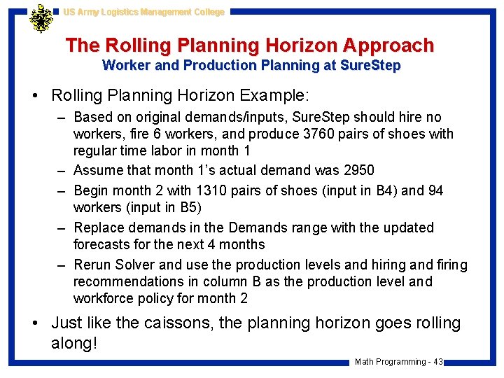
US Army Logistics Management College The Rolling Planning Horizon Approach • In reality, an aggregate planning model is usually implemented via a rolling planning horizon • Let’s assume that Sure. Step works with a 4 -month planning horizon • To implement the Sure. Step model in the rolling planning horizon context: – View the “demands” as forecasts and solve a 4 -month model with these forecasts – Implement only the month 1 production and work scheduling recommendation – Observe month 1’s actual demand ending inventory and workers available. – Input inventory and worker results from month 1 in cells B 4 & B 5 – Replace demands in the Demands range with the updated forecasts for the next 4 months and resolve Math Programming - 42

US Army Logistics Management College The Rolling Planning Horizon Approach Worker and Production Planning at Sure. Step • Rolling Planning Horizon Example: – Based on original demands/inputs, Sure. Step should hire no workers, fire 6 workers, and produce 3760 pairs of shoes with regular time labor in month 1 – Assume that month 1’s actual demand was 2950 – Begin month 2 with 1310 pairs of shoes (input in B 4) and 94 workers (input in B 5) – Replace demands in the Demands range with the updated forecasts for the next 4 months – Rerun Solver and use the production levels and hiring and firing recommendations in column B as the production level and workforce policy for month 2 • Just like the caissons, the planning horizon goes rolling along! Math Programming - 43

US Army Logistics Management College Modeling Issues Worker and Production Planning at Sure. Step 1. Hiring costs include training costs as well as the cost of decreased productivity due to the fact that a new worker must learn his or her job 2. Firing costs include severance costs and costs due to loss of morale 3. Peterson and Silver recommend that when demand is seasonal, the planning horizon should extend beyond the next seasonal peak 4. Beyond a certain point, the cost of using extra hours of overtime labor increases because workers become less efficient Math Programming - 44

US Army Logistics Management College Minimum Cost Network Flow Models Producing and Shipping Tomato Products at Red. Brand Math Programming - 45

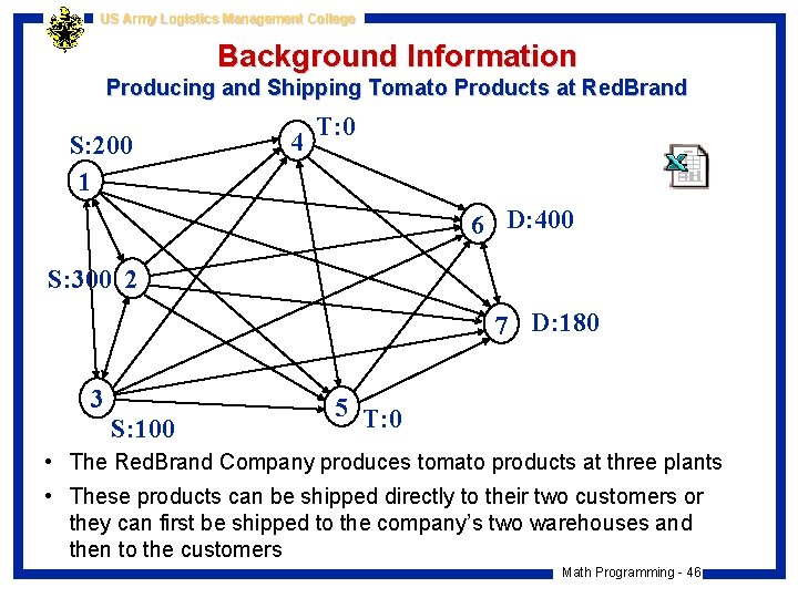
US Army Logistics Management College Background Information Producing and Shipping Tomato Products at Red. Brand S: 200 1 4 T: 0 6 D: 400 S: 300 2 7 D: 180 3 S: 100 5 T: 0 • The Red. Brand Company produces tomato products at three plants • These products can be shipped directly to their two customers or they can first be shipped to the company’s two warehouses and then to the customers Math Programming - 46

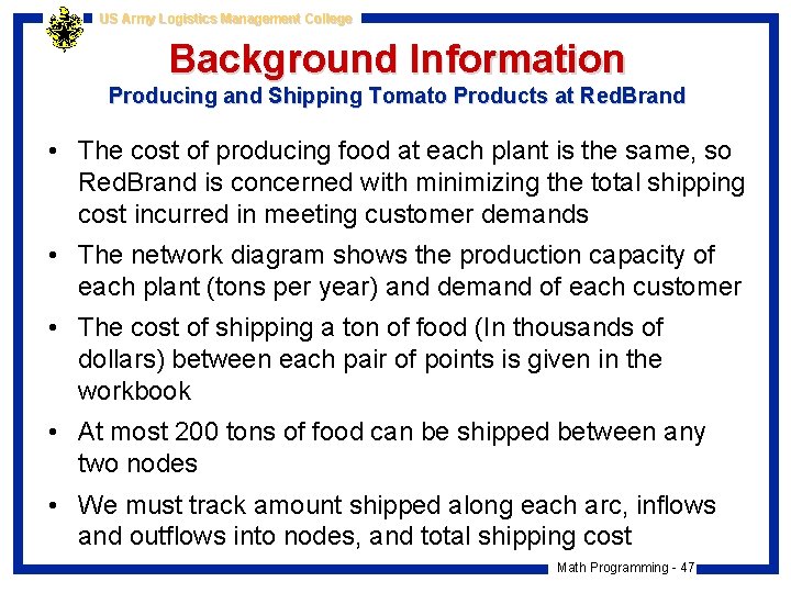
US Army Logistics Management College Background Information Producing and Shipping Tomato Products at Red. Brand • The cost of producing food at each plant is the same, so Red. Brand is concerned with minimizing the total shipping cost incurred in meeting customer demands • The network diagram shows the production capacity of each plant (tons per year) and demand of each customer • The cost of shipping a ton of food (In thousands of dollars) between each pair of points is given in the workbook • At most 200 tons of food can be shipped between any two nodes • We must track amount shipped along each arc, inflows and outflows into nodes, and total shipping cost Math Programming - 47

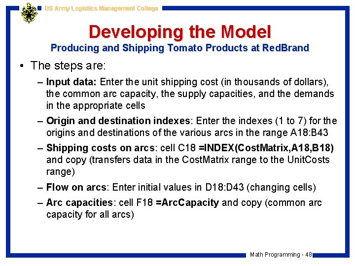
US Army Logistics Management College Developing the Model Producing and Shipping Tomato Products at Red. Brand • The steps are: – Input data: Enter the unit shipping cost (in thousands of dollars), the common arc capacity, the supply capacities, and the demands in the appropriate cells – Origin and destination indexes: Enter the indexes (1 to 7) for the origins and destinations of the various arcs in the range A 18: B 43 – Shipping costs on arcs: cell C 18 =INDEX(Cost. Matrix, A 18, B 18) and copy (transfers data in the Cost. Matrix range to the Unit. Costs range) – Flow on arcs: Enter initial values in D 18: D 43 (changing cells) – Arc capacities: cell F 18 =Arc. Capacity and copy (common arc capacity for all arcs) Math Programming - 48

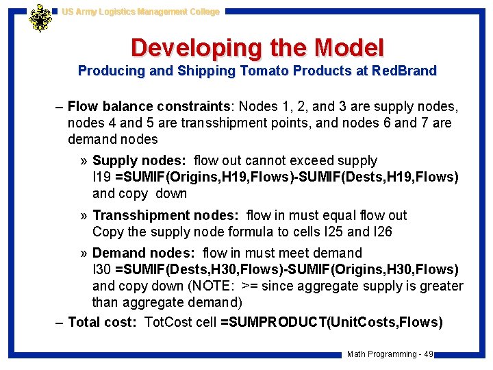
US Army Logistics Management College Developing the Model Producing and Shipping Tomato Products at Red. Brand – Flow balance constraints: Nodes 1, 2, and 3 are supply nodes, nodes 4 and 5 are transshipment points, and nodes 6 and 7 are demand nodes » Supply nodes: flow out cannot exceed supply I 19 =SUMIF(Origins, H 19, Flows)-SUMIF(Dests, H 19, Flows) and copy down » Transshipment nodes: flow in must equal flow out Copy the supply node formula to cells I 25 and I 26 » Demand nodes: flow in must meet demand I 30 =SUMIF(Dests, H 30, Flows)-SUMIF(Origins, H 30, Flows) and copy down (NOTE: >= since aggregate supply is greater than aggregate demand) – Total cost: Tot. Cost cell =SUMPRODUCT(Unit. Costs, Flows) Math Programming - 49

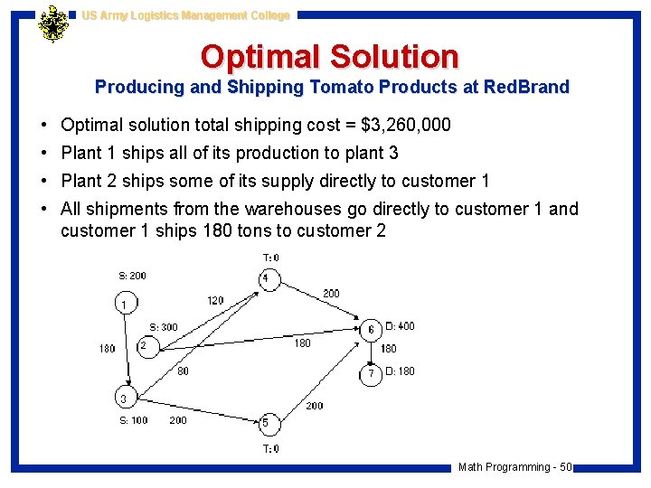
US Army Logistics Management College Optimal Solution Producing and Shipping Tomato Products at Red. Brand • Optimal solution total shipping cost = $3, 260, 000 • Plant 1 ships all of its production to plant 3 • Plant 2 ships some of its supply directly to customer 1 • All shipments from the warehouses go directly to customer 1 and customer 1 ships 180 tons to customer 2 Math Programming - 50

US Army Logistics Management College Sensitivity Analysis Producing and Shipping Tomato Products at Red. Brand • How much effect does the arc capacity have on optimal solution? – Currently, three arcs with positive flow are at the arc capacity of 200 – Use Solver. Table to see how a change in arc capacity effects the shipping pattern and total cost – The single input cell is the Arc. Capacity cell (vary from 150 to 300 in increments of 25) – Track two outputs: total cost and number of arcs at capacity [arc capacity: C 47 =COUNTIF(Flows, Arc. Capacity) ] – As arc capacity decreases, more flows bump up against it, and total cost increases – Even at an arc capacity is 300, up to two flows are constrained (multi-optimal solutions) Math Programming - 51

US Army Logistics Management College Model Variation: Multi-product Producing and Shipping Tomato Products at Red. Brand • Suppose Red. Brand ships two products along the given network – Assume that the unit shipping costs are the same for either product – The arc capacity represents the maximum flow of both products that can flow on any arc (the two products are competing for arc capacity) – Each plant has a separate production capacity for each product and each customer has a separate demand for each product Math Programming - 52

US Army Logistics Management College Multi-product Model Formulation Producing and Shipping Tomato Products at Red. Brand • Very little needs to be changed from the original model • If you rename cells appropriately, the Solver dialog box does not have to be changed • Changes to the original model: – have two columns of changing cells – apply the previous logic to both products separately in the flow balance constraints – apply the arc capacities to the total flows in column F Math Programming - 53

US Army Logistics Management College Model Variation: Flow loss Model Producing and Shipping Tomato Products at Red. Brand • A second variation of the model is appropriate for perishable goods • Assume that there is a single product, but that some percentage of the product that is shipped to warehouses perishes and cannot be sent on to customers • Having this flow loss means that the total inflow to a warehouse is greater than the total outflow from the warehouse Math Programming - 54

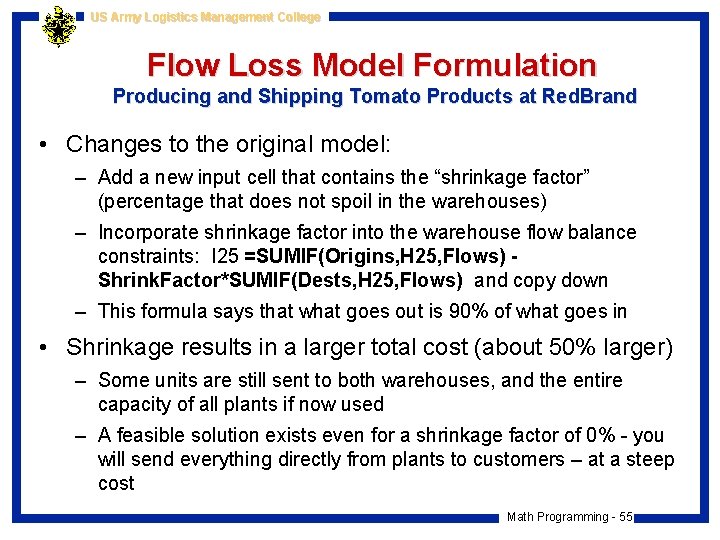
US Army Logistics Management College Flow Loss Model Formulation Producing and Shipping Tomato Products at Red. Brand • Changes to the original model: – Add a new input cell that contains the “shrinkage factor” (percentage that does not spoil in the warehouses) – Incorporate shrinkage factor into the warehouse flow balance constraints: I 25 =SUMIF(Origins, H 25, Flows) Shrink. Factor*SUMIF(Dests, H 25, Flows) and copy down – This formula says that what goes out is 90% of what goes in • Shrinkage results in a larger total cost (about 50% larger) – Some units are still sent to both warehouses, and the entire capacity of all plants if now used – A feasible solution exists even for a shrinkage factor of 0% - you will send everything directly from plants to customers – at a steep cost Math Programming - 55

US Army Logistics Management College Math Programming Integer Programming and Multi-objective Models Math Programming - 56

US Army Logistics Management College Plant and Warehouse Location Models Facility Location and Logistics Planning at Huntco Math Programming - 57

US Army Logistics Management College Background Information Facility Location and Logistics Planning at Huntco • • Huntco produces tomato sauce at five different plants. Each plant has a finite supply capacity (in tons). The tomato sauce is stored at one of three warehouses. Huntco has four customers that receive shipments from the warehouses based on their demand. • Costs incurred include: – production and shipping costs from plant to warehouse – Shipping costs from warehouse to customer – Plant and warehouse operating costs (annual fixed amount) • Huntco’s goal is to minimize the annual cost of meeting customer demands. • The company wants to determine which plants and warehouses to open, as well as the optimal shipping plan. Math Programming - 58

US Army Logistics Management College Modeling Approach Facility Location and Logistics Planning at Huntco • To model Huntco’s problem, we need to track: – – – Shipments from plants to warehouses Shipments from warehouses to customers Fixed costs of operating plants and warehouses Shipping and production costs from plants to warehouses Shipping costs from warehouses to customers Total amount shipped out of each plant • We must also ensure that – Huntco pays the fixed costs for all plants and warehouses that it uses. – The amount shipped into each warehouse equals the amount received by each warehouse. – Each customer receives the specified demand. Math Programming - 59

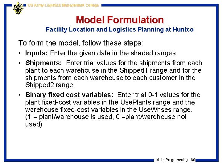
US Army Logistics Management College Model Formulation Facility Location and Logistics Planning at Huntco To form the model, follow these steps: • Inputs: Enter the given data in the shaded ranges. • Shipments: Enter trial values for the shipments from each plant to each warehouse in the Shipped 1 range and for the shipments from each warehouse to each customer in the Shipped 2 range. • Binary fixed cost variables: Enter trial 0 -1 values for the plant fixed-cost variables in the Use. Plants range and the warehouse fixed-cost variables in the Use. Whses range. (1 = plant/warehouse is used, 0 =plant/warehouse not used) Math Programming - 60

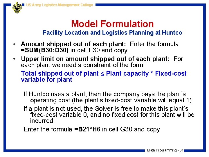
US Army Logistics Management College Model Formulation Facility Location and Logistics Planning at Huntco • Amount shipped out of each plant: Enter the formula =SUM(B 30: D 30) in cell E 30 and copy • Upper limit on amount shipped out of each plant: For each plant we need a constraint of the form Total shipped out of plant Plant capacity * Fixed-cost variable for plant If Huntco uses a plant, then the company pays the plant’s operating cost (the plant’s fixed-cost variable will equal 1) If a plant is not used, the Solver is free to make this plant’s fixed-cost variable 0, and no fixed cost for this plant will be incurred. Enter the formula =B 21*H 6 in cell G 30 and copy Math Programming - 61

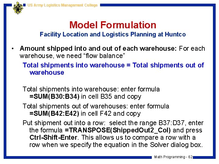
US Army Logistics Management College Model Formulation Facility Location and Logistics Planning at Huntco • Amount shipped into and out of each warehouse: For each warehouse, we need “flow balance” Total shipments into warehouse = Total shipments out of warehouse Total shipments into warehouse: enter formula =SUM(B 30: B 34) in cell B 35 and copy Total shipments out of warehouses: enter formula =SUM(B 42: E 42) in cell F 42 and copy Put shipment out into a row: select the range B 37: D 37, enter the formula =TRANSPOSE(Shipped. Out 2_Col) and press Ctrl-Shift-Enter. This allows us to compare a row with a row when we specify the equation in the Solver dialog box. Math Programming - 62

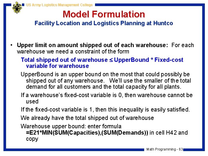
US Army Logistics Management College Model Formulation Facility Location and Logistics Planning at Huntco • Upper limit on amount shipped out of each warehouse: For each warehouse we need a constraint of the form Total shipped out of warehouse Upper. Bound * Fixed-cost variable for warehouse Upper. Bound is an upper bound on the most that could possibly be shipped out of any warehouse. We’ll use the smaller of the total demand for all customers and the total capacity for all plants. If a warehouse’s fixed-cost variable is 0, then warehouse cannot be used If the fixed-cost variable is 1, then this inequality is easily satisfied. We already have the total shipped out of warehouse Warehouse upper bound: enter formula =E 21*MIN(SUM(Capacities), (SUM(Demands)) in cell H 42 and copy Math Programming - 63

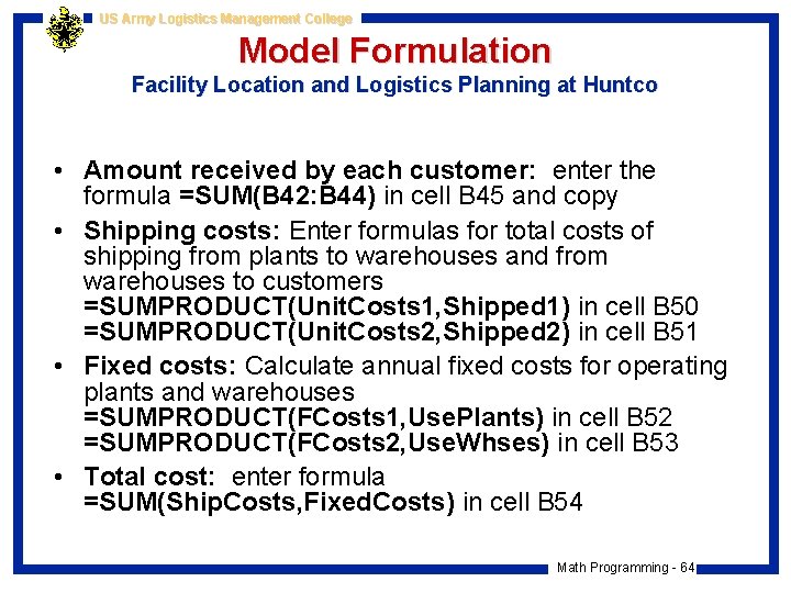
US Army Logistics Management College Model Formulation Facility Location and Logistics Planning at Huntco • Amount received by each customer: enter the formula =SUM(B 42: B 44) in cell B 45 and copy • Shipping costs: Enter formulas for total costs of shipping from plants to warehouses and from warehouses to customers =SUMPRODUCT(Unit. Costs 1, Shipped 1) in cell B 50 =SUMPRODUCT(Unit. Costs 2, Shipped 2) in cell B 51 • Fixed costs: Calculate annual fixed costs for operating plants and warehouses =SUMPRODUCT(FCosts 1, Use. Plants) in cell B 52 =SUMPRODUCT(FCosts 2, Use. Whses) in cell B 53 • Total cost: enter formula =SUM(Ship. Costs, Fixed. Costs) in cell B 54 Math Programming - 64

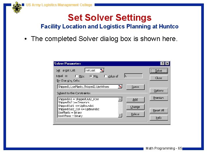
US Army Logistics Management College Set Solver Settings Facility Location and Logistics Planning at Huntco • The completed Solver dialog box is shown here. Math Programming - 65

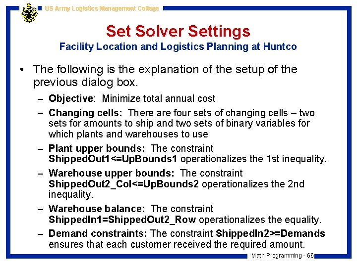
US Army Logistics Management College Set Solver Settings Facility Location and Logistics Planning at Huntco • The following is the explanation of the setup of the previous dialog box. – Objective: Minimize total annual cost – Changing cells: There are four sets of changing cells – two sets for amounts to ship and two sets of binary variables for which plants and warehouses to use – Plant upper bounds: The constraint Shipped. Out 1<=Up. Bounds 1 operationalizes the 1 st inequality. – Warehouse upper bounds: The constraint Shipped. Out 2_Col<=Up. Bounds 2 operationalizes the 2 nd inequality. – Warehouse balance: The constraint Shipped. In 1=Shipped. Out 2_Row operationalizes the equality. – Demand constraints: The constraint Shipped. In 2>=Demands ensures that each customer received the required amount. Math Programming - 66

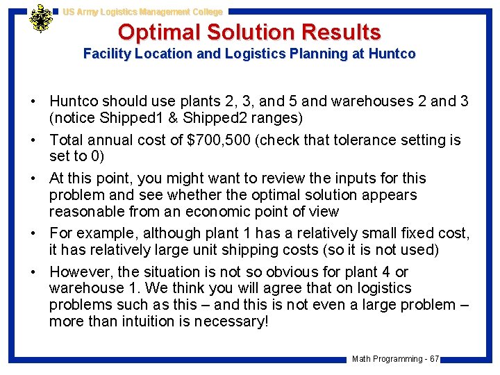
US Army Logistics Management College Optimal Solution Results Facility Location and Logistics Planning at Huntco • Huntco should use plants 2, 3, and 5 and warehouses 2 and 3 (notice Shipped 1 & Shipped 2 ranges) • Total annual cost of $700, 500 (check that tolerance setting is set to 0) • At this point, you might want to review the inputs for this problem and see whether the optimal solution appears reasonable from an economic point of view • For example, although plant 1 has a relatively small fixed cost, it has relatively large unit shipping costs (so it is not used) • However, the situation is not so obvious for plant 4 or warehouse 1. We think you will agree that on logistics problems such as this – and this is not even a large problem – more than intuition is necessary! Math Programming - 67

US Army Logistics Management College Sensitivity Analysis Facility Location and Logistics Planning at Huntco • We will not report any specific sensitivity analyses for this model, but many are possible. – For example, we might check whether adding larger capacities at plants 1 and 4 would induce Huntco to open them. – Or we might see what would happen if all the fixed costs increases by some percentage. – Or we might see what would happen if all customer demands increased by some percentage. • Solver. Table, after some slight model modifications, can easily analyze any of these situations. Math Programming - 68

US Army Logistics Management College Models with Either-Or Constraints Manufacturing at Dorian Auto Math Programming - 69

US Army Logistics Management College Background Information Manufacturing at Dorian Auto • Dorian Auto is considering manufacturing three types of cars – compact, midsize, and large • Each car type uses steel and labor resources and earns a profit • At present, 6000 tons of steel and 60, 000 hours of labor are available • If any cars of a given type are produced, production of that type of car will be economically feasible only if at least 1000 cars of that type are produced • Dorian wants to find a production schedule that maximizes its profit Math Programming - 70

US Army Logistics Management College Model Formulation Manufacturing at Dorian Auto • In addition to tracking the number of each car type produced, labor hours, steel used, and profit, we must ensure that Dorian produces either 0 or at least 1000 cars of each type – this is an either-or constraint • To develop the model, follow these steps: • Inputs: Enter the input data into the shaded ranges • Numbers of cars produced: Enter trial values for the number of cars of each type produced in the Units. Produced range • Binary variables for minimum production: Enter any trial 0 -1 values in the Produce. Min range (1=Dorian must produce at least the minimum number of the corresponding car type, 0=do not produce any of that type car) Math Programming - 71

US Army Logistics Management College Model Formulation Manufacturing at Dorian Auto • The either-or constraints are implemented with the binary variables in row 13 and the inequalities in rows 15 and 19 • Lower limits on production: enter the formula =B 7*B 13 in cell B 15 and copy (if the binary variable in row 13 = 1, then produce at least the minimum number of that car type, if the binary variable = 0, then the lower bound is 0 and production must be nonnegative) • Upper limits on production: enter the formula =B 13*MIN(Steel. Avail/B 5, Labor. Avail/B 6) in cell B 19 and copy - the MIN term in this formula is the max number of type cars Dorian could make if it devoted all of its resources to that type car - If the binary variable in row 13 is 1, this upper limit is essentially redundant – we could never produce more than this many cars - If the binary variable is 0, then the upper limit is 0, which prevents Dorian from making any cars of this type Math Programming - 72

US Army Logistics Management College Model Formulation Manufacturing at Dorian Auto • Summarizing the lower & upper limits, if the binary variable is 1, the production limits become Min production required Production Maxproduction possible • If the binary variable is 0, the limits become 0 Production 0 • Exactly one of these cases must hold for each car type, so they successfully implement the either-or constraints • Steel / labor used: enter the formula =SUMPRODUCT(B 5: D 5, Units. Produced) in cell B 22 and copy to calculate the tons of steel and number of labor hours used • Profit: Calculate the profit in the Profit cell with the formula =SUMPRODUCT(Unit. Profits, Units. Produced). Math Programming - 73

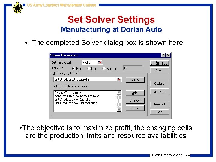
US Army Logistics Management College Set Solver Settings Manufacturing at Dorian Auto • The completed Solver dialog box is shown here • The objective is to maximize profit, the changing cells are the production limits and resource availabilities Math Programming - 74

US Army Logistics Management College Optimal Solution Manufacturing at Dorian Auto • The optimal solution shown in the earlier figure indicates, by the 0 values in row 13, that Dorian should not produce any compact or large cars • The value of 1 in cell C 13, however, indicates that Dorian must produce at least the minimum number, 1000, of midsize cars • Actually, midsize cars are quite profitable, so Dorian produces as many as possible, 2000, before running into the steel availability constraint Math Programming - 75

US Army Logistics Management College Sensitivity Analysis Manufacturing at Dorian Auto • What type of incentive might cause the company to produce more than one car type? – One possible answer is that the minimum production levels for each type, all currently 1000, are perhaps too high – Use Solver. Table to see the effect of decreasing each of these minimum production levels by the same factor (the model must be modified slightly: go to the worksheet labeled Sensitivity) – Input the original minimum production levels in range F 5: H 5, and enter the formula =Decr. Factor*H 5 in cell B 7 and copy it across row 7 – Invoke Solver. Table with the Decr. Factor cell as the single input cell, varied from 0. 2 to 1 in increments of 0. 2, and keep track of profit and all changing cell values Math Programming - 76

US Army Logistics Management College Sensitivity Analysis Manufacturing at Dorian Auto • Solver. Table results indicate that when the minimum production levels are reduced to 200 or 400, Dorian produces both compact and midsize cars above the minimum level • When the minimum production level is 600, Dorian still produces both types, but it does not produce any more compacts than necessary • Finally, when the minimum production level is 800 or 1000, Dorian produces only midsize cars – as many as steel availability allows • Does this sound correct? We checked it, and it is correct, but here is a test of your economic reasoning • The results seems to imply that compacts extract less profit from the resources than midsize cars. But if this is the case, why doesn’t Dorian produce the minimum number of compacts when the minimum production is 200 or 400? (for example, when it is 400, why doesn’t Dorian produce 400 compacts and 1800 midsize cars? ) Math Programming - 77

US Army Logistics Management College Goal Programming Determining an Advertising Schedule at Leon Burnit Math Programming - 78

US Army Logistics Management College Background Information Determining an Advertising Schedule at Leon Burnit • The Leon Burnit Ad Agency is trying to determine a TV advertising schedule for a client • The client has three goals (listed in descending order of importance) – Goal 1: at least 65 million high-income men (HIM) – Goal 2: at least 72 million high-income women (HIW) – Goal 3: at least 70 million low-income people (LP) • Burnit can purchase ads to air on different program types (live sports shows, game shows, news shows, sitcoms, dramas, and soap operas), each with different ad costs & audience makeup • At most $700, 000 total can be spent on ads • The client requires that at least two ads be placed on sports shows, news shows, and dramas, and that no more than ten ads be placed on any single type of show • Burnit wants to find the advertising plan that best meets its client’s goals Math Programming - 79

US Army Logistics Management College Solution Approach Determining an Advertising Schedule at Leon Burnit • First, we build a spreadsheet model to see whether all of the goals can be met simultaneously. • In the spreadsheet model we must keep track of the following: – The number of ads placed for each show type – The cost of the ads – The number of exposures to each group (HIM, HIW, LIP) – The deviation from the exposure goal of each group Math Programming - 80

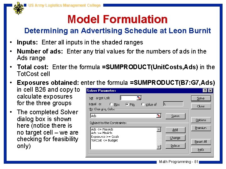
US Army Logistics Management College Model Formulation Determining an Advertising Schedule at Leon Burnit • Inputs: Enter all inputs in the shaded ranges • Number of ads: Enter any trial values for the numbers of ads in the Ads range • Total cost: Enter the formula =SUMPRODUCT(Unit. Costs, Ads) in the Tot. Cost cell • Exposures obtained: enter the formula =SUMPRODUCT(B 7: G 7, Ads) in cell B 26 and copy to calculate exposures for the three groups • The completed Solver dialog box is shown here (notice there is no target cell – we are checking for feasibility only) Math Programming - 81

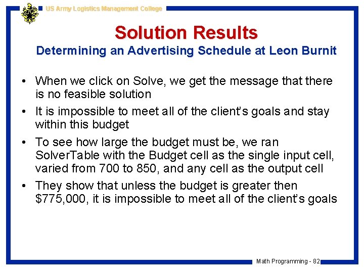
US Army Logistics Management College Solution Results Determining an Advertising Schedule at Leon Burnit • When we click on Solve, we get the message that there is no feasible solution • It is impossible to meet all of the client’s goals and stay within this budget • To see how large the budget must be, we ran Solver. Table with the Budget cell as the single input cell, varied from 700 to 850, and any cell as the output cell • They show that unless the budget is greater then $775, 000, it is impossible to meet all of the client’s goals Math Programming - 82

US Army Logistics Management College Goal Programming Determining an Advertising Schedule at Leon Burnit • Since a $700, 000 budget is not sufficient to meet all of the client’s goals, use goal programming to see how close Burnit can come to their goals • The upper and lower limits on the ads of each type and the budget constraints are considered hard constraints in this model (they cannot be violated under any circumstances) • The goals on exposures, on the other hand, are considered soft constraints (the client wants to satisfy these goals, but it is willing to come up somewhat short – in fact, it must because of the limited budget) • In goal programming models the soft constraints are prioritized – We first try to satisfy the goals with the highest priority – If there is still any room to maneuver, we then try to satisfy the goals with the next highest priority – If there is still room to maneuver, we move on to the goals with the third highest priority, and so on Math Programming - 83

US Army Logistics Management College Goal Programming Model Determining an Advertising Schedule at Leon Burnit • In general, goal programming requires several consecutive Solver runs, one for each priority level • However, it is possible to set up the model so that we can make these consecutive runs with only minor changes from one run to the next (use the worksheet Goal Programming) • New changing cells: We additional changing cells in the Dev. Under and Dev. Over ranges (Dev is short for “deviations”) to indicate how much or over each goal we are In the solution • At least one of these two types of deviations will always be 0 for each goal – we will either be below the goal or above the goal, but not both Math Programming - 84

US Army Logistics Management College Goal Programming Model Determining an Advertising Schedule at Leon Burnit • Balance equations: enter the formula =B 26+C 26 -D 26 in cell E 26 and copy to tie the deviation cells to the rest of the model • The balance equation for each group specifies that the actual number of exposures plus the number under the goal minus the number over the goal (Col E) must be equal the goal (Col G) • Constraints on deviations under: enter the formula =C 26 in cell B 32 and copy to measure the “under” deviations • The client is concerned only with too few exposures, not with too many Math Programming - 85

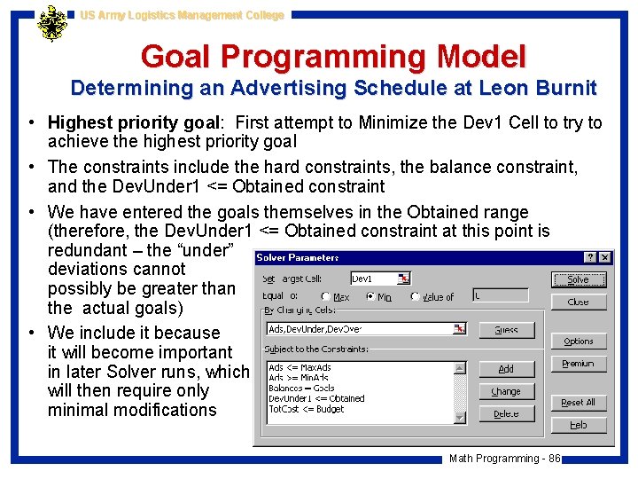
US Army Logistics Management College Goal Programming Model Determining an Advertising Schedule at Leon Burnit • Highest priority goal: First attempt to Minimize the Dev 1 Cell to try to achieve the highest priority goal • The constraints include the hard constraints, the balance constraint, and the Dev. Under 1 <= Obtained constraint • We have entered the goals themselves in the Obtained range (therefore, the Dev. Under 1 <= Obtained constraint at this point is redundant – the “under” deviations cannot possibly be greater than the actual goals) • We include it because it will become important in later Solver runs, which will then require only minimal modifications Math Programming - 86

US Army Logistics Management College Goal Programming Model Determining an Advertising Schedule at Leon Burnit • The solution shows that Burnit can satisfy the HIM goal completely (the other two goals are not satisfied because their “under” deviations are positive) • Second highest priority goal: Now we come to the key aspect of goal programming – Once a high priority goal is satisfied as fully as possible, we move on to the next highest priority goal – Constrain the “under” deviation for the first goal to be no greater than what we already achieved (we achieved a deviation of 0 for HIM, so enter 0 in cell D 32) – Run the Solver again, changing only the target cell in to Dev 2 (we are minimizing the “under” deviation for the HIW group) Math Programming - 87

US Army Logistics Management College Goal Programming Model Determining an Advertising Schedule at Leon Burnit • The solution from this second Solver run shows that the HIM goal has not suffered at all, but we are now a little closer to the HIW goal than before (it was under 11. 75 before, and now it is under by only 11) • The lowest priority goal get worse, moving from under by 11. 25 to under by 18 (it could either improve or get worse) • Lowest priority goal: Minimize the Dev 3 cell, the deviation for the LIP group, while ensuring that the two higher priority goals are achieved (make sure cell D 32=0 and cell D 33=11) Math Programming - 88

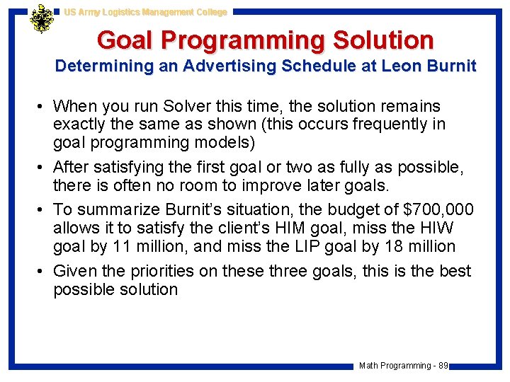
US Army Logistics Management College Goal Programming Solution Determining an Advertising Schedule at Leon Burnit • When you run Solver this time, the solution remains exactly the same as shown (this occurs frequently in goal programming models) • After satisfying the first goal or two as fully as possible, there is often no room to improve later goals. • To summarize Burnit’s situation, the budget of $700, 000 allows it to satisfy the client’s HIM goal, miss the HIW goal by 11 million, and miss the LIP goal by 18 million • Given the priorities on these three goals, this is the best possible solution Math Programming - 89

US Army Logistics Management College Sensitivity Analysis Determining an Advertising Schedule at Leon Burnit • There is no quick way to do sensitivity analysis on a goal programming model • Solver. Table works on only a single objective, whereas goal programming requires a sequence of objectives • If we want to see how the solution to Burnit’s model changes with different budget levels, we would need to go through the above steps several times and keep track of the results manually Math Programming - 90

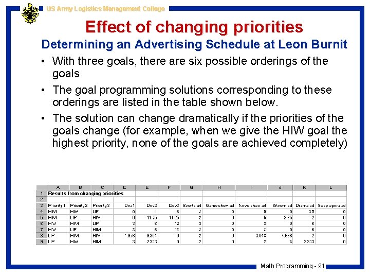
US Army Logistics Management College Effect of changing priorities Determining an Advertising Schedule at Leon Burnit • With three goals, there are six possible orderings of the goals • The goal programming solutions corresponding to these orderings are listed in the table shown below. • The solution can change dramatically if the priorities of the goals change (for example, when we give the HIW goal the highest priority, none of the goals are achieved completely) Math Programming - 91

US Army Logistics Management College Pareto Optimality and Trade-off Curves Maximizing Profit and Minimizing Pollution at Chemcon Math Programming - 92

US Army Logistics Management College Background Information Max Profit and Min Pollution at Chemcon • Chemcon plans to produce eight products, each with different requirements for labor, raw materials, min and max production levels, and profit margins • Currently 1300 labor hours and 1000 units of raw material are available • Chemcon’s two objectives are to maximize profit and minimize pollution produced • Chemcon wants to graph the trade-off curve for this problem Math Programming - 93

US Army Logistics Management College Developing a Trade-Off Curve Max Profit and Min Pollution at Chemcon • We want the product mix that stays within the lower and upper production limits, uses no more labor or raw material than are available, keeps pollution low, and keeps profit high • To develop a trade-off curve, we let profit be objective 1 and pollution be objective 2 • To obtain one endpoint of the curve, we maximize profit and ignore pollution (maximize the Profit cell and delete the Pollution constraint) • The optimal solution had profit $20, 089 and pollution level 8980 Math Programming - 94

US Army Logistics Management College Developing a Trade-Off Curve Max Profit and Min Pollution at Chemcon • At the other extreme, we can minimize the pollution in cell B 26 and ignore any constraint on profit • You can check that this solution has pollution level 3560 and profit $8360 • Profit can get as high as $20, 089 by ignoring pollution or as low as $8360 by focusing entirely on pollution, and pollution can get as low as 3560 by ignoring profit or as high as 8980 by focusing entirely on profit • These establish the extremes - now we can search for points in between Math Programming - 95

US Army Logistics Management College Developing a Trade-Off Curve Max Profit and Min Pollution at Chemcon • To develop the trade-off curve, we will add the pollution constraint back into the model and use Solver. Table • We need to constrain pollution to various degrees and see how large profit can be • This is indicated in the model, where the objective is to maximize profit with an upper limit on pollution • The only upper limits on pollution we need to consider are those between the extremes, 3560 and 8980 Math Programming - 96

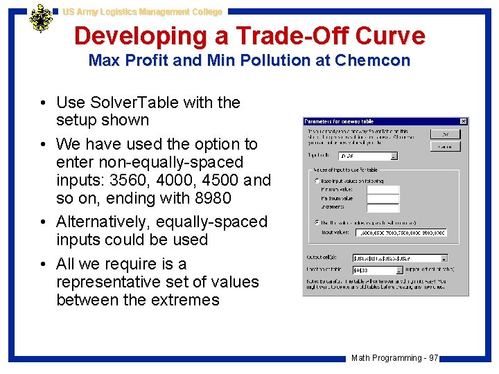
US Army Logistics Management College Developing a Trade-Off Curve Max Profit and Min Pollution at Chemcon • Use Solver. Table with the setup shown • We have used the option to enter non-equally-spaced inputs: 3560, 4000, 4500 and so on, ending with 8980 • Alternatively, equally-spaced inputs could be used • All we require is a representative set of values between the extremes Math Programming - 97

US Army Logistics Management College Developing a Trade-Off Curve Max Profit and Min Pollution at Chemcon • These results show that as we allow more pollution, profit increases (the product mix also shifts considerably) • Profit 8, a low polluter with a low profit margin, eventually leaves the mix when pollution is allowed to increase, which makes sense • It is less clear why the level of product 6 increases so dramatically (it is only a moderate polluter and has a moderate profit margin, so the key is evidently that it requires low levels of labor and raw materials. ) • The trade-off curve is created as an X_Y chart directly from columns J and K of the table Math Programming - 98

US Army Logistics Management College Developing a Trade-Off Curve Max Profit and Min Pollution at Chemcon • The chart indicates that profit indeed increases as Chemcon allows more pollution, but at a decreasing rate • For example, when pollution is allowed to increase from 4000 to 4500, Chemcon can make an extra $3187 in profit • However, when pollution is allowed to increase from 8000 to 8500, the extra profit is only $532 • All points below the curve are dominated – for a given level of pollution, the company can achieve a larger profit – and all points above the curve are unattainable Math Programming - 99