URBAN STORMWATER DRAINAGE A typical gully pit URBAN

URBAN STORMWATER DRAINAGE A typical gully pit

URBAN STORMWATER DRAINAGE When the design fails!

URBAN STORMWATER DRAINAGE Design of urban stormwater drainage involves Ø Hydrologic calculations of catchment flow rates Ø Hydraulic calculations of pit energy and friction losses, and pipe sizes

URBAN STORMWATER DRAINAGE Hydraulic Design
 Ø Friction slope Pipe slope Ø Allow 150")
URBAN STORMWATER DRAINAGE Hydraulic Design (continue) Ø Friction slope Pipe slope Ø Allow 150 mm freeboard for USWL & DSWL Ø USWL - DSWL Losses Ø Losses = Friction + Pit energy losses Ø Calculate pipe size to satisfy above condition


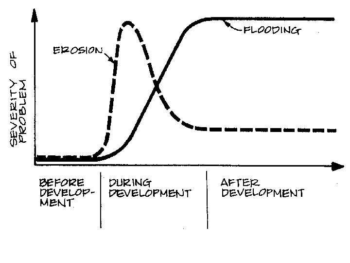
If we completely fill in the floodplain and develop every bit of space, this is what we get Lincoln Creek in Milwaukee

Channel enlarged because there is no flood plain

A solution - picks up 96% of solids. Cost effective

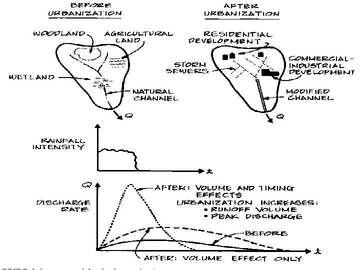
before after

Total annual precipitation In WI = approx. 30 in no connection no reduction a/b b a
")
Example of Roof Runoff Into Trench (CT)
")
Parking Lot Infiltration Systems (CT)
")
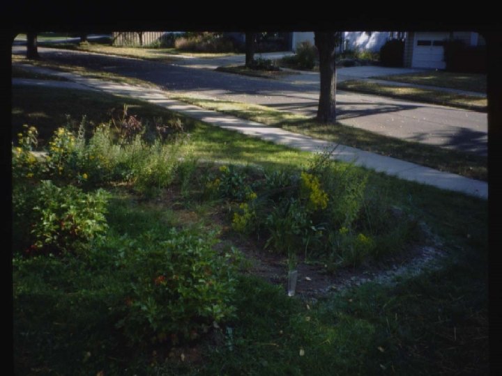
Grass Swales (Waukesha County)
")
Rain Island (MD)
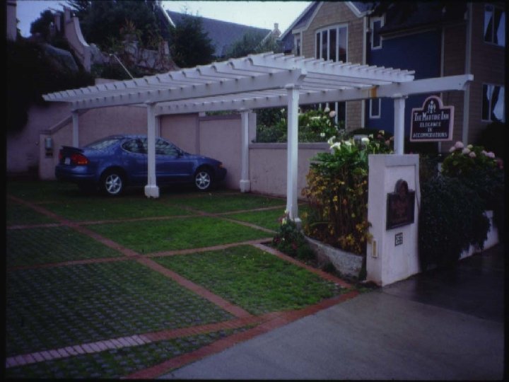

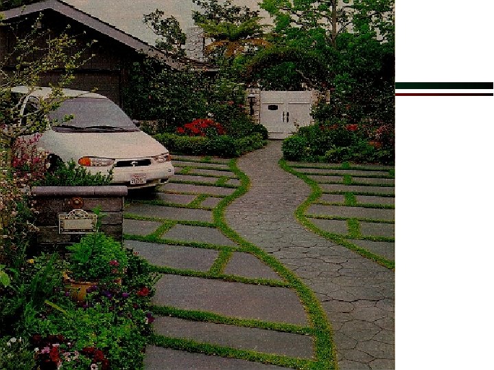
Red Cross Headquarters In Madison

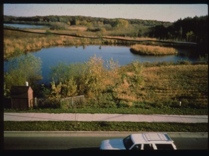
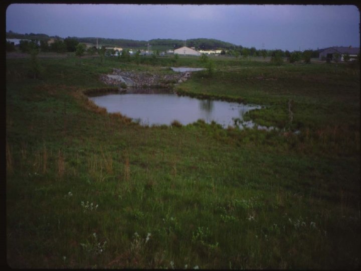
Natural Wetland Detention Design


Hydrology Ø Meteorology Ø Study of the atmosphere including weather and climate Ø Surface water hydrology Ø Flow and occurrence of water on the surface of the earth Ø Hydrogeology Ø Flow and occurrence of ground water

Engineering Uses of Surface Water Hydrology Ø Average events (average annual rainfall, evaporation, infiltration. . . ) Ø Expected average performance of a system Ø Potential water supply using reservoirs Ø Frequent extreme events (10 year flood, 10 year low flow) Ø Levees Ø Wastewater dilution Ø Rare extreme events (100 to PMF) Ø Dam failure Ø Power plant flooding Probable maximum flood

Flood Design Techniques Ø Use stream flow records Ø Limited data Ø Can be used for high probability events Ø Use precipitation records Ø Use rain gauges rather than stream gauges Ø Determine flood magnitude based on precipitation, runoff, streamflow Ø Create a synthetic storm Ø Based on record of storms

Sources of Data Ø Stream flows Ø tamab Ø Precipitation Ø tamab Ø National Weather Service Ø Global extreme events

Forecasting Stream Flows Ø Natural processes not easily predicted in a deterministic way 10 year daily average Ø We cannot predict the monthly stream flow Ø We will use probability distributions instead of predictions Seasonal trend with large variation

Choice of Return Periods: RISK!!! Ø How do you choose an acceptable risk? Potential harm Acceptable risk Ø Crops Ø Parking lot Ø Water treatment plant Ø Nuclear power plant Ø Large dam Ø What about long term changes? Ø Global climate change Ø Development in the watershed Ø Construction of Levees

Design Flood Exceedance Ø Example: what is the probability that a 100 year design flood is exceeded at least once in a 50 year project life (small dam design) Not (safe for 50 years) Ø =___________ (p = probability of exceedance in one year) probability of safe performance for one year probability of safe performance for two years probability of safe performance for n years probability of exceedance in n years probability that 100 year flood exceeded at least once in 50 years

Empirical Estimation of 10 Year Flood Ø Sort annual max discharge in decreasing order Annual Peak Flow Record How often was data collected? 10 year flood Ø Plot vs. Where N is the number of years in the record 2 year flood

Extreme Events Ø Suppose we can only accept a 1% chance of failure due to flooding in a 50 year project life. What is the return period for the design flood? Ø Given 50 year project life, 1% chance of failure requires the probability of exceedance to be _____ 0. 02% in one year Ø Extreme event! Return period of _____ 5000 years!

Extreme Events Ø Low probability of failure requires the probability of failure in one year to be very low Ø The design event has most likely not occurred in the historic record Ø Nuclear power plant on bank of river ØDesigned for flood with 100, 000 year return period, but have observations for 100 years

Quantifying Extreme Events Ø Use stream flow records to describe distribution including skewness and then extrapolate Ø Adjust gage station flows to project site based on watershed area Ø Use similar adjacent watersheds if stream flow data is unavailable for the project stream Ø Use rainfall data and apply a model to estimate stream flow Ø Use local rain gage data Ø Use global maximum precipitation Ø Estimate probable maximum precipitation for the site

Flood Design Process Ø Create a synthetic storm Ø Estimate the infiltration, depression storage, and runoff Ø Estimate the stream flow We need models!
 hydrology ØBased on physical principles ØMechanistic description")
Methods to Predict Runoff Ø Scientific (dynamic) hydrology ØBased on physical principles ØMechanistic description ØDifficult given all the local details Ø Engineering (empirical) hydrology Ø“Rational formula” ØSoil cover complex method ØMany others
 Hydrology Ø Based on observations and experience Ø Overall description without attempt")
Engineering (Empirical) Hydrology Ø Based on observations and experience Ø Overall description without attempt to describe details Ø Mostly concerned with various methods of estimating or predicting precipitation and streamflow

p. 359 in Chin “Rational Formula” Ø Qp = Ci. A Ø QP = peak runoff Ø C is a dimensionless coefficient ØC=f(land use, slope) Øhttp: //ceeserver. Cee. Cornell. Edu/mw 24/cee 3 32/scs_cn/runoff_coefficients. Htm Ø i = rainfall intensity [L/T] Ø A = drainage area [L 2]
 Ø Expectation")
“Rational Formula” Method to Choose Rainfall Intensity Ø Intensity = f(storm duration) Ø Expectation of stream flow vs. Time during storm of constant intensity Q Qp Watershed divide Outflow point tc t
 Ø Time required (after start of rainfall event)")
“Rational Formula” Time of Concentration (Tc) Ø Time required (after start of rainfall event) for most distant point in basin to begin contributing runoff to basin outlet Ø Tc affects the shape of the outflow hydrograph (flow record as a function of time)
![Time of Concentration (Tc): Kirpich Ø Tc = time of concentration [min] Ø L](http://slidetodoc.com/presentation_image_h2/abb2d8e4d7d2f91d75c7350ffadf34ff/image-45.jpg "Time of Concentration (Tc): Kirpich Ø Tc = time of concentration [min] Ø L")
Time of Concentration (Tc): Kirpich Ø Tc = time of concentration [min] Ø L = “stream” or “flow path” length [ft] Ø h = elevation difference between basin ends [ft] Watch those units!
![Time of Concentration (Tc): Hatheway Ø Tc = time of concentration [min] Ø L](http://slidetodoc.com/presentation_image_h2/abb2d8e4d7d2f91d75c7350ffadf34ff/image-46.jpg "Time of Concentration (Tc): Hatheway Ø Tc = time of concentration [min] Ø L")
Time of Concentration (Tc): Hatheway Ø Tc = time of concentration [min] Ø L = “stream” or “flow path” length [ft] Ø S = mean slope of the basin Ø N = Manning’s roughness coefficient (0. 02 smooth to 0. 8 grass overland)

“Rational Formula” Review Ø Estimate tc Ø Pick duration of storm = tc. Why is the max flow? Ø Estimate point rainfall intensity based on synthetic storm Ø Convert point rainfall intensity to average area intensity Ø Estimate runoff coefficient based on land use

“Rational Formula” Fall Creek 10 Year Storm Ø C 0. 25 (moderately steep, grass covered clayey soils, some development) Runoff Coefficients Ø Qp = Ci. A Ø QP = 7300 ft 3/s (200 m 3/s) Ø Empirical 10 year flood is approximately 150 m 3/s

“Rational Method” Limitations Ø Reasonable for small watersheds < 80 ha Ø The runoff coefficient is not constant during a storm Ø No ability to predict flow as a function of time (only peak flow) Ø Only applicable for storms with duration longer than the time of concentration
 Ø Create a synthetic storm Ø Estimate infiltration and runoff")
Flood Design Process (Review) Ø Create a synthetic storm Ø Estimate infiltration and runoff ØSoil cover complex Ø Estimate the streamflow Ø“Rational method” ØHydrographs

Not stream flow! Runoff As a Function of Rainfall Ø Exercise: plot cumulative runoff vs. Cumulative precipitation for a parking lot and for the engineering quad. Assume a rainfall of 1/2” per hour for 10 hours. Accumulated runoff Parking lot ? Accumulated rainfall Engineering Quad

Infiltration Ø Water filling soil pores and moving down through soil Ø Depends on soil type and grain size, land use and soil cover, and antecedent moisture conditions (prior to rainfall) Ø Usually maximum at beginning of storm (dry soils, large pores) and decreases as moisture content increases Ø Vegetation (soil cover) prevents soil compaction by rainfall and increases infiltration
 “curve number” method")
Soil Cover Complex Method Ø US NRCS (Natural Resources Conservation Service) “curve number” method Ø Accounts for Ø Initial abstraction of rainfall before runoff begins Ø Interception Ø Depression storage Ø Infiltration after runoff begins Ø Appropriate for small watersheds
 is a value assigned to different")
Soil Cover Complex Method Ø CN (curve number) is a value assigned to different soil types based on Ø Soil type Ø Land use Ø Antecedent conditions f(initial moisture content) Ø CN (curve number) range Ø 0 to 100 (actually %) Ø 0 low runoff potential Ø 100 high runoff potential
 Ø Land use Ø")
CN = F(soil Type, Land Use, Hydrologic Condition, Antecedent Moisture) Ø Land use Ø Crop type Ø Woods Ø Roads antecedent moisture I dry soil moisture levels II normal soil moisture levels III wet soil moisture levels Ø Hydrologic condition Ø Poor heavily grazed, less than 50% plant cover Ø Fair moderately grazed, 50 75% plant cover Ø Good lightly grazed, more than 75% plant cover
 rain that will")
Soil Cover Complex Method Ø pexcess = accumulated precipitation excess (inches) rain that will become runoff Ø P = accumulated precipitation depth (inches) Ø Empirical equation if else then

Soil Cover Complex Method: Graph Parking lot

Soil cover Complex Method Ø Choose CN based on soil type, land use, hydrologic condition, antecedent moisture Ø Subareas of the basin can have different CN Ø Compute area weighted averages for CN Ø Choose storm event (precipitation vs. time) Ø Calculate cumulative rainfall excess vs. time Ø Calculate incremental rainfall excess vs. time (to get runoff produced vs. time)

Stream Flow Ø Runoff vs. Time ___ stream flow vs. Time Ø Water from different points will arrive at gage station at different times Ø Need a method to convert runoff into stream flow

Hydrographs Ø Graph of stream flow vs. time Ø Obtained by means of a continuous recorder which indicates stage vs. time (stage hydrograph) Ø Transformed to a discharge hydrograph by application of a rating curve Ø Typically are complex multiple peak curves Ø Available on the web Real Hydrographs

Hydrographs Ø Introduction ØThere are many types of hydrographs ØI will present one type as an example ØThis is a science with lots of art! Ø Assumptions ØLinearity hydrographs can be superimposed ØPeak discharge is proportional to runoff rate* * Required for linearity

Hydrograph Nomenclature storm of Duration D Precipitation P tl tp peak flow Discharge Q baseflow new baseflow w/o rainfall Time
")
NRCS* Dimensionless Unit Hydrograph Q/Qp Ø Unit = 1 inch of runoff (not rainfall) in 1 hour Ø Can be scaled to other depths and times Ø Based on unit hydrographs from many watersheds 1. 000 0. 800 0. 600 0. 400 0. 200 0. 000 0 * Natural Resources Conservation Service 1 2 3 t/tp 4 5

NRCS Dimensionless Unit Hydrograph Tp the time from the beginning of the rainfall to peak discharge [hr] Tl the lag time from the centroid of rainfall to peak discharge [hr] D the duration of rainfall [hr] (D < 0. 25 tl) (use sequence of storms of short duration) Qp peak discharge [cfs] A drainage area [mi 2] L length to watershed divide in feet S average watershed slope CN NRCS curve number

Storm Hydrograph Ø Calculate incremental runoff for each hour during storm using soil cover complex method Ø Scale NRCS dimensionless unit hydrograph by ØPeak flow ØTime to peak ØRunoff depth for each hour (relative to 1 inch) Ø Add unit hydrographs for each hour of the storm (shifted in time) to get storm hydrograph
 = 24 m 3/s")
Addition of Hydrographs Qmax = 0. 2(4200 cfs) = 24 m 3/s

What are NRCS Limitations? Ø No snow melt Ø No rain on snow Ø Lumped model (infiltration/runoff over entire watershed is characterized by a single number) Ø Stream flow model is simplistic (reduced to a time of concentration)
 Ø Extrapolate")
Hydrology Summary Ø Techniques to predict stream flows Ø Historical record (USGS) Ø Extrapolate from adjoining watersheds Ø Estimate based on precipitation Rainfall Runoff Stream Flow Rain gages Synthetic Storm Rational Method NRCS Soil Cover Complex Method NRCS Hydrograph


/www. dfo-mpo. gc. ca/canwaters-eauxcan/infocentre/guidelines-conseils/factsheets-feuillets/nfld/images/fact 17_e/4 -7. jpg 70

Detention Basin Purposes Ø Store water temporarily during a storm and release the stored water slowly Ø Attenuate the flow Ø Store first flush Ø Design for infiltration ØIf all water is infiltrated then (retention basin) 71

Detention Basins Ø On Site Ø Regional 72
 Ø Storage Ø Outflow (single/multiple stage ØOrifice")
Detention Basins Ø Inflow (ditch or pipe) Ø Storage Ø Outflow (single/multiple stage ØOrifice ØWeir Ø Emergency spillway 73

Routing Ø Method used to model the outflow hydrograph Ø Based on continuity equation ØWater in varies ØWater out varies 74

Information Needed to Route Ø Inflow hydrograph Ø Relation of storage volume to elevation in the proposed detention basin Ø Relation of outflow to water level elevation (discharge rating) 75
 Ø Modified rational method")
Inflow hydrograph Ø Ch 5 of TR 55 (NRCS method) Ø Modified rational method ØSimple symmetrical triangle (2*tc) ØAsymmetrical triangle (total base = 2. 67 tc) 76
 Peak flow is higher after development Peak flow occurs")
TR 55 Hydrograph (NRCS Method) Peak flow is higher after development Peak flow occurs earlier after development

Rational Method: Simple Symmetrical Triangle

Rational Method: Area under hydrograph? Time base of 2. 67 tc
 ØAverage End Area (pipes)")
Computing Storage Volumes Ø Two Methods ØElevation Area (detention basins) ØAverage End Area (pipes) 80
 ØContour lines are determined around basin")
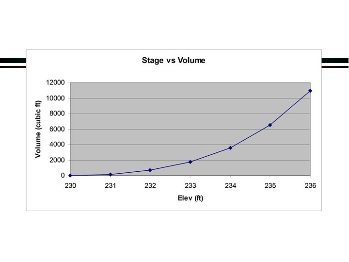
Computing Storage Volumes Ø Elevation Area (detention basins) ØContour lines are determined around basin ØDetermine area of each contour ØVolume between 2 contours = average area*depth between the contours ØPrepare a table showing elevation, area, incremental volume and cumulative volume ØSee example 14 1 (page 341) 81
 Area (ft 2) Incr. Vol (ft")
Elevation Area Method: Ex 14 1 Elev (ft) Area (ft 2) Incr. Vol (ft 3) 230 0 231 250 232 840 233 Cum. Vol (ft 3) 0 0 125 545 670 1350 1095 1765 234 2280 1815 3580 235 3680 2980 6560 236 5040 4360 10, 920 (250/2*1)= ((250+840)/2*1)=
- Slides: 83