Update on Lightning Mapping Systems using the New

Update on Lightning Mapping Systems using the New Mexico Tech Lightning Mapping Array Bill Rison, Paul Krehbiel, and Ron Thomas New Mexico Tech, Socorro, New Mexico

Lightning Mapping Arrays • Langmuir Lab (Experimental) • North Alabama (NASA) • Oklahoma (OU/NSSL) • White Sands (Army) • Portable

CG Flash example, 2004 Compact LMA, Langmuir Lab 10 microsecond windows

Portable LMA ● 18 Stations, Rapid Deployment ● No Central Station or Real-Time Processing ● Powered from +12 V DC, ~12 W ● For use in Short-Term Field Programs ● Construction to be Finished in Fall, 2005

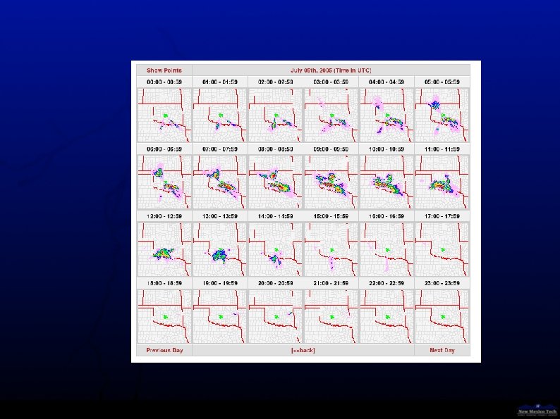
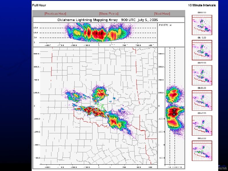
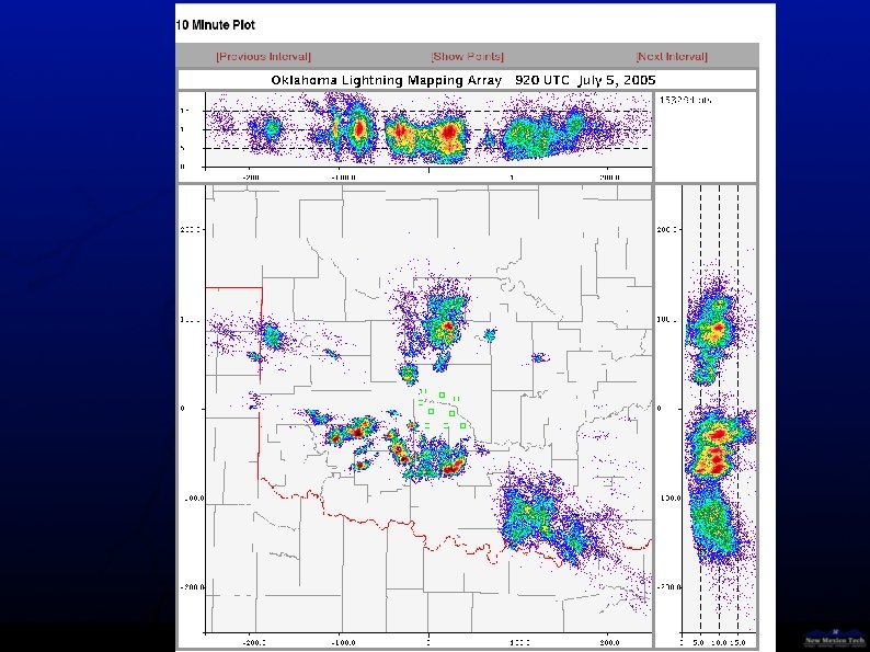
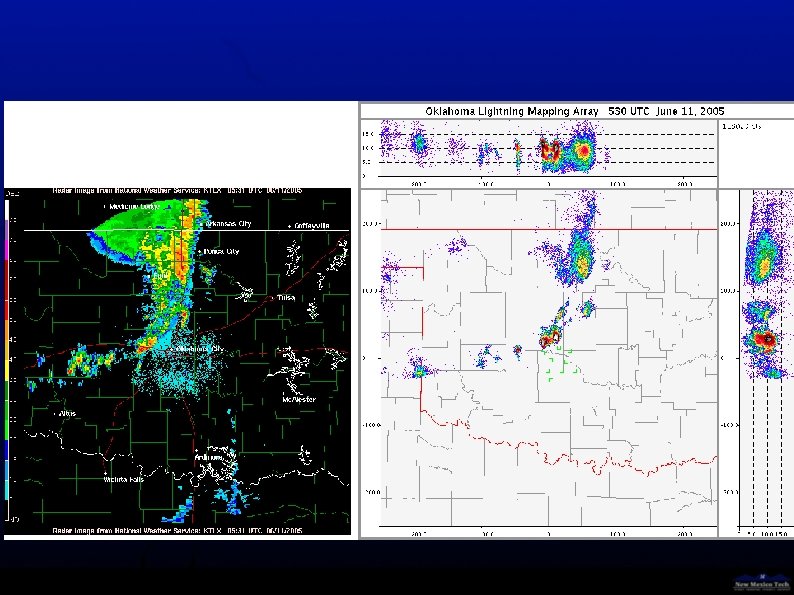
University of Oklahoma/National Severe Storms Laboratory

802. 11 b Wireless Network Eight station daisy-chain through Goldsby

Real-Time Data Transfer ● Real-Time Data in One Minute Packets ● All stations try to send data at same time ● Interference between wireless channels results in loss of data packets – ● More loss during intense lightning periods Needed to find more robust way to transfer data

Leapfrog Data – Two Minutes Max Time Delay Robust Transfer – Almost no Loss of Data

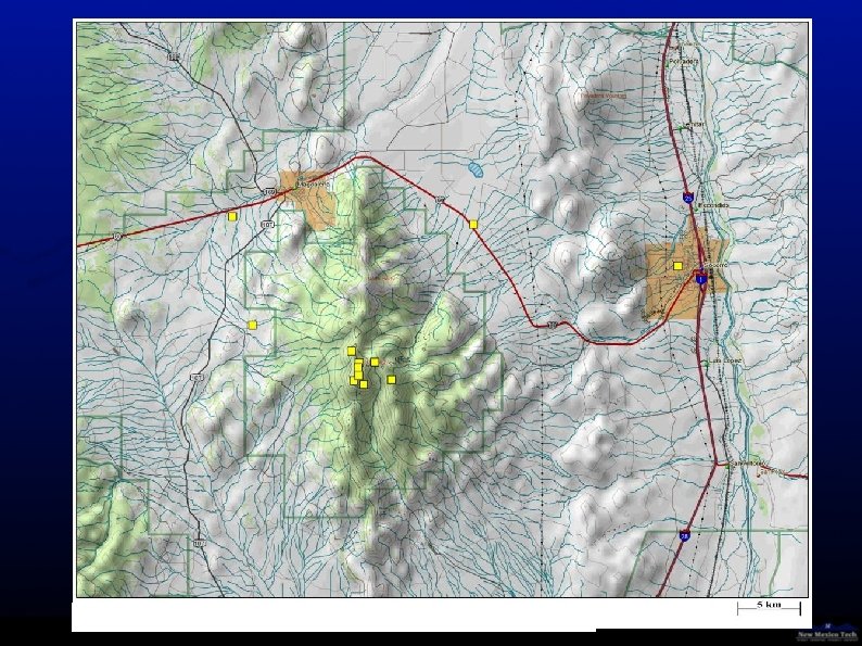
LMA – Radar Comparison

White Sands LMA Twelve Station Network ●Fiber Optic Communications ●First data – 8 Stations, 7/14/05 ●NCAR to incorporate into Auto-nowcasting ●

“First Lightning” from WSMR LMA

NMT Focus ● Continued Development of Systems – Improved Hardware – Real-Time Processing and Display ● Helping in Operation of Oklahoma LMA ● Developing New Processing Code ● Continued Development of XLMA

Issues Concerning Uniformity of Data ● System Parameters – Noise Levels – Number of Stations – Decimation Levels – Robustness of Real-Time Data Transfer ● Range Dependence ● Processing Code ● Source Density vs Flash Extent/Density

New Processing Code • Written in C++ As before: • Processes 1 sec of data at a time, • Arrival times ('trigger events') ordered chronologically in a 1 -D array • Go sequentially through the array, event by event, • Assume the current event is the first event of an actual source, • Search only forward in time for other triggers that could correspond • to the initial trigger,

Sample Combination Sequence

Scatter diagram of c*Delta t vs. chi square for different combinations (some repeated)

Metric vs. chisqr for the different combinations metric = (c*dt)*(parabolic chisq weight)

Combination solutions (black dots) overlaid on overall results (turquoise) Selected solution (red) Selected solution – red (plan view)

Vertical projections of combination results (Selected solution in red) (Selected solution consistent with overall results)

Metric vs. combination sequence number (note repeated solutions) ('Stop early' after 5 repeats of low metric value)

Scatter diagram of c*Delta t vs. chi square (more complex, 11 -station example) (Lowest c*dt is 11 -station solution with chisqr = 1. 8 - black circle)

Chisqr-weighted metric: Selects 10 -station solution with chisqr < 1 (red) Chi-square weighting function: [1 + (chisq^2)/4]

Comparison of selected result (red) overall results (turqoise) – Plan view

Vertical projection comparisons (selected solution in red) (Selected solution consistent with overall results)

Metric vs. combination sequence number (5 repeats found after 13/108 combinations) (Stop early saves processing time & picks best solution)

Original vs. new processing code: ~3 times faster; obtain better solutions (involving more stations) This example: Fewer solutions with new code due to narrower window for getting 6 or more stations (200 ns vs 2. 7 microseconds) –> increased noise immunity.

Original vs. new processing code: North Alabama LMA 0221 2005, 2020: 00 -01 Slightly greater number of solutions, located with more stations

CG Flash example, 2004 Compact LMA, Langmuir Lab 10 microsecond windows

IC Flash example, 2004 Compact LMA, Langmuir Lab 10 microsecond windows