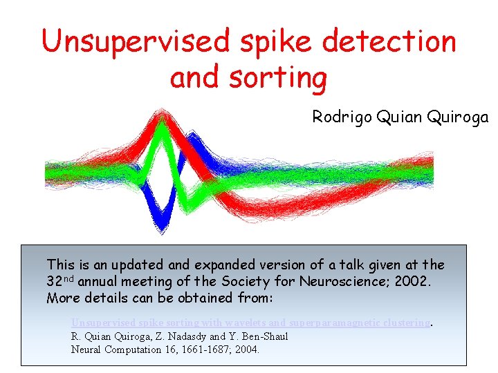
Unsupervised spike detection and sorting Rodrigo Quian Quiroga

Unsupervised spike detection and sorting Rodrigo Quian Quiroga This is an updated and expanded version of a talk given at the 32 nd annual meeting of the Society for Neuroscience; 2002. More details can be obtained from: Unsupervised spike sorting with wavelets and superparamagnetic clustering. R. Quian Quiroga, Z. Nadasdy and Y. Ben-Shaul Neural Computation 16, 1661 -1687; 2004.

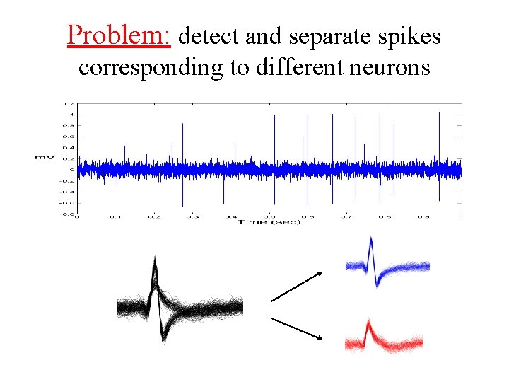
Problem: detect and separate spikes corresponding to different neurons

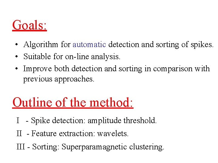
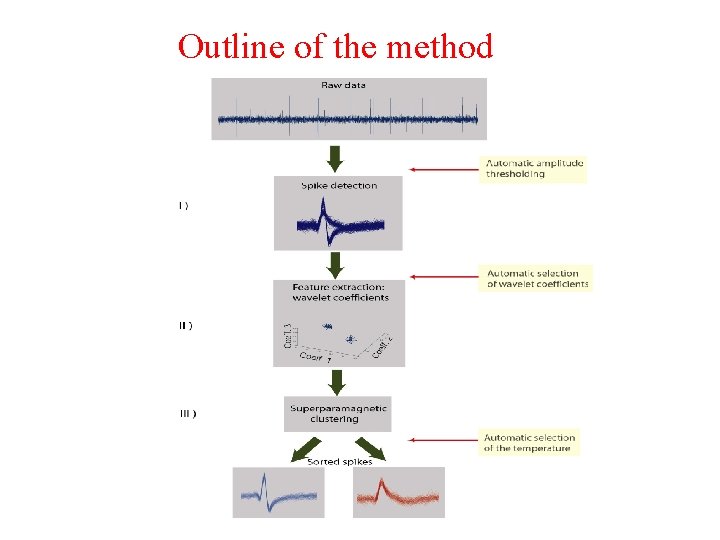
Goals: • Algorithm for automatic detection and sorting of spikes. • Suitable for on-line analysis. • Improve both detection and sorting in comparison with previous approaches. Outline of the method: I - Spike detection: amplitude threshold. II - Feature extraction: wavelets. III - Sorting: Superparamagnetic clustering.

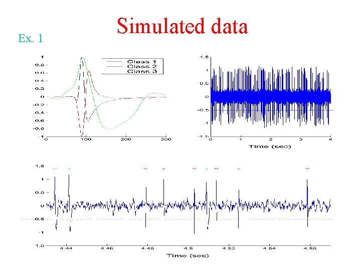
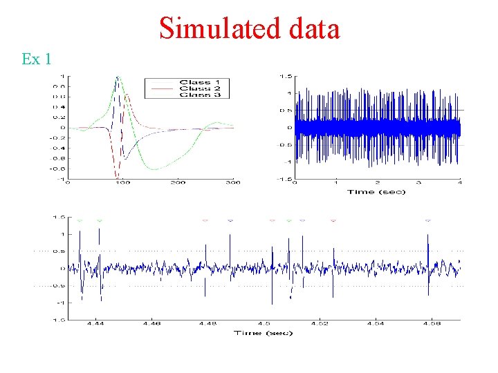
Ex. 1 Simulated data

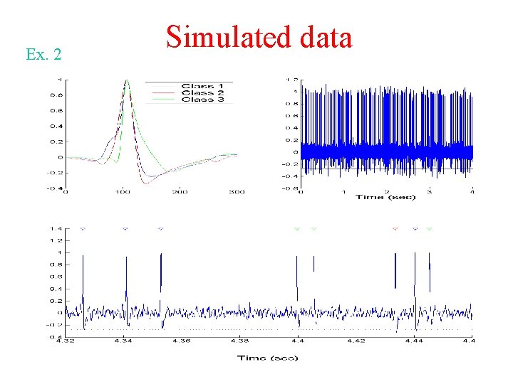
Ex. 2 Simulated data

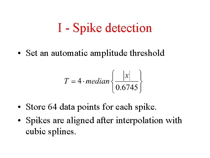
I - Spike detection • Set an automatic amplitude threshold • Store 64 data points for each spike. • Spikes are aligned after interpolation with cubic splines.

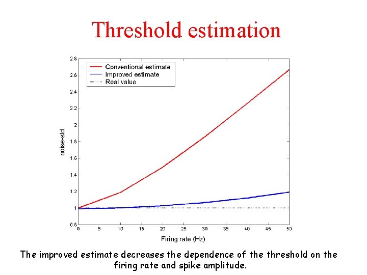
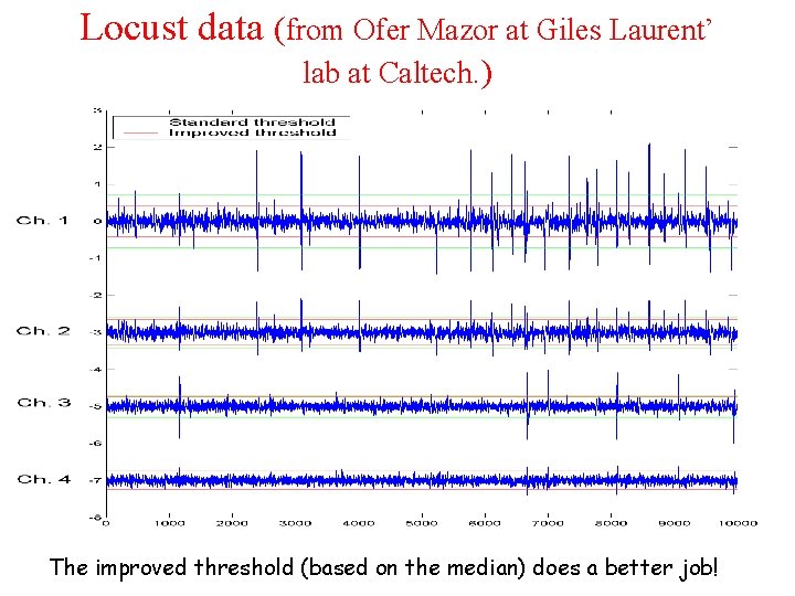
Threshold estimation The improved estimate decreases the dependence of the threshold on the firing rate and spike amplitude.

Detection results (in brackets, results including overlapping spikes). Example # [noise level] Nr. of spikes Misses False positives Ex. 1 [0. 05] 3514 (785) 17 (193) 711 [0. 10] 3522 (769) 2 (177) 57 [0. 15] 3477 (784) 145 (215) 14 [0. 20] 3474 (796) 714 (275) 10 Ex. 2 [0. 05] 3410 (791) 0 (174) 0 [0. 10] 3520 (826) 0 (191) 2 [0. 15] 3411 (763) 10 (173) 1 [0. 20] 3526 (811) 376 (256) 5 Ex. 3 [0. 05] 3383 (767) 1 (210) 63 [0. 10] 3448 (810) 0 (191) 10 [0. 15] 3472 (812) 8 (203) 6 [0. 20] 3414 (790) 184 (219) 2 Ex. 4 [0. 05] 3364 (829) 0 (182) 1 [0. 10] 3462 (720) 0 (152) 5 [0. 15] 3440 (809) 3 (186) 4 [0. 20] 3493 (777) 262 (228) 2

II - Feature extraction: wavelets

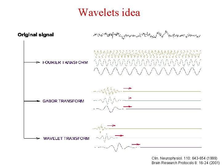
Wavelets idea Clin. Neurophysiol. 110: 643 -654 (1999) Brain Research Protocols 8: 16 -24 (2001)

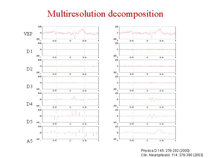
Multiresolution decomposition VEP D 1 D 2 D 3 D 4 D 5 A 5 Physica D 145: 278 -292 (2000) Clin. Neurophysiol. 114: 376 -390 (2003)

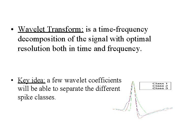
• Wavelet Transform: is a time-frequency decomposition of the signal with optimal resolution both in time and frequency. • Key idea: a few wavelet coefficients will be able to separate the different spike classes.

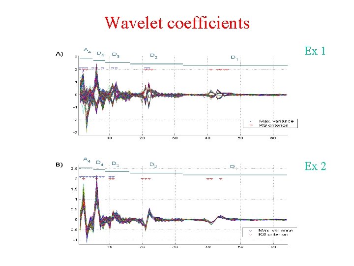
Wavelet coefficients Ex 1 Ex 2

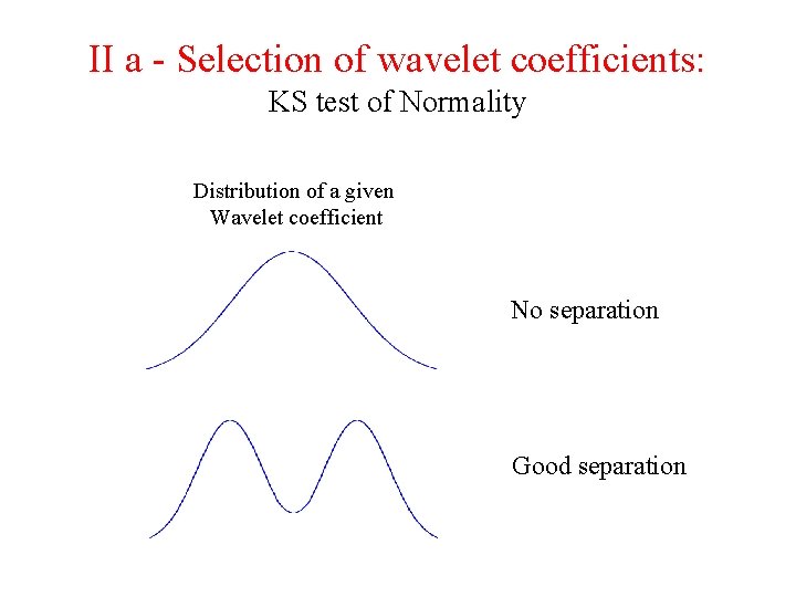
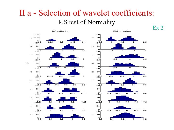
II a - Selection of wavelet coefficients: KS test of Normality Distribution of a given Wavelet coefficient No separation Good separation

II a - Selection of wavelet coefficients: KS test of Normality Ex 2

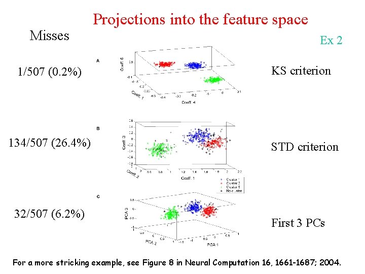
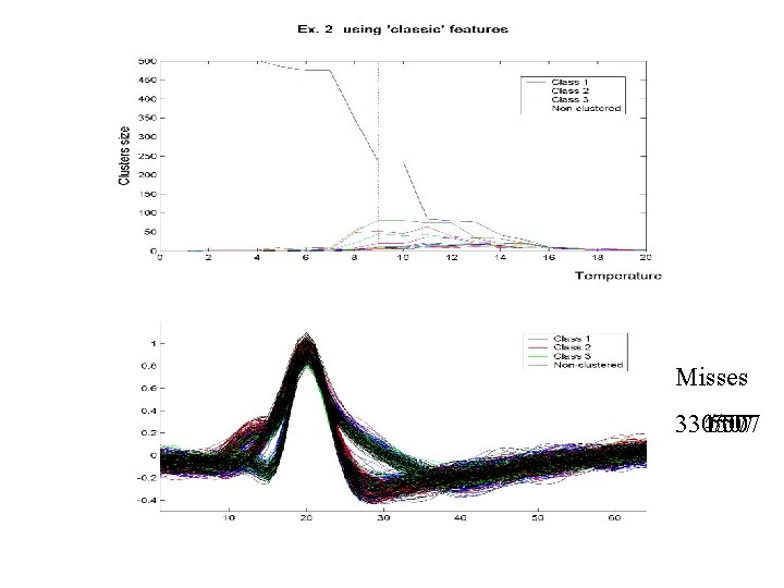
Misses 1/507 (0. 2%) 134/507 (26. 4%) 32/507 (6. 2%) Projections into the feature space Ex 2 KS criterion STD criterion First 3 PCs For a more stricking example, see Figure 8 in Neural Computation 16, 1661 -1687; 2004.

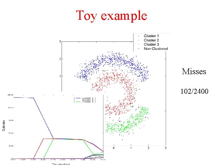
III – Superparamagnetic clustering • Automatic clustering algorithm based on ideas from statistical mechanics. • It’s based on nearest-neighbor’s interactions. • Clusters don’t need to have a well-defined center, low variance or a Gaussian distribution.

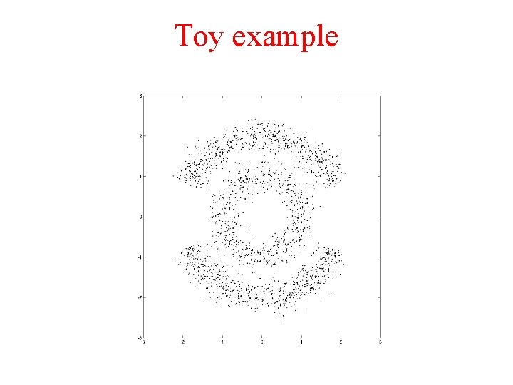
Toy example

Toy example Misses 102/2400

Outline of the method

Simulated data Ex 1

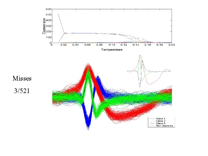
Misses 3/521

Ex. 2 Simulated data

Misses 134/507 330/507 32/507 1/507

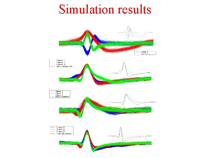
Simulation results

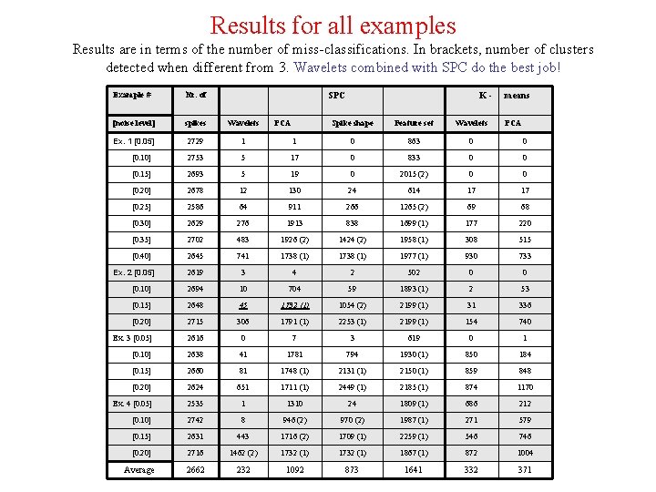
Results for all examples Results are in terms of the number of miss-classifications. In brackets, number of clusters detected when different from 3. Wavelets combined with SPC do the best job! Example # Nr. of [noise level] spikes Wavelets Ex. 1 [0. 05] 2729 1 [0. 10] 2753 [0. 15] SPC means Spike shape Feature set Wavelets 1 0 863 0 0 5 17 0 833 0 0 2693 5 19 0 2015 (2) 0 0 [0. 20] 2678 12 130 24 614 17 17 [0. 25] 2586 64 911 266 1265 (2) 69 68 [0. 30] 2629 276 1913 838 1699 (1) 177 220 [0. 35] 2702 483 1926 (2) 1424 (2) 1958 (1) 308 515 [0. 40] 2645 741 1738 (1) 1977 (1) 930 733 2619 3 4 2 502 0 0 [0. 10] 2694 10 704 59 1893 (1) 2 53 [0. 15] 2648 45 1732 (1) 1054 (2) 2199 (1) 31 336 [0. 20] 2715 306 1791 (1) 2253 (1) 2199 (1) 154 740 Ex. 3 [0. 05] 2616 0 7 3 619 0 1 [0. 10] 2638 41 1781 794 1930 (1) 850 184 [0. 15] 2660 81 1748 (1) 2131 (1) 2150 (1) 859 848 [0. 20] 2624 651 1711 (1) 2449 (1) 2185 (1) 874 1170 Ex. 4 [0. 05] 2535 1 1310 24 1809 (1) 686 212 [0. 10] 2742 8 946 (2) 970 (2) 1987 (1) 271 579 [0. 15] 2631 443 1716 (2) 1709 (1) 2259 (1) 546 746 [0. 20] 2716 1462 (2) 1732 (1) 1867 (1) 872 1004 Average 2662 232 1092 873 1641 332 371 Ex. 2 [0. 05] PCA K- PCA

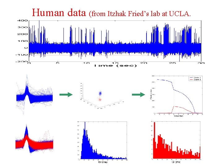
Human data (from Itzhak Fried’s lab at UCLA.

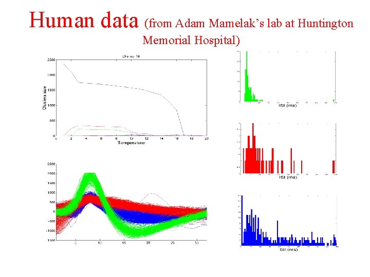
Human data (from Adam Mamelak’s lab at Huntington Memorial Hospital)

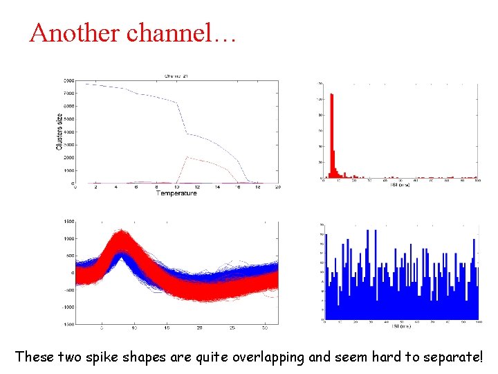
Another channel… These two spike shapes are quite overlapping and seem hard to separate!

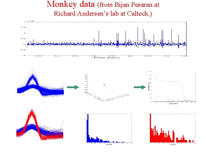
Monkey data (from Bijan Pesaran at Richard Andersen’s lab at Caltech. )

Locust data (from Ofer Mazor at Giles Laurent’ lab at Caltech. ) The improved threshold (based on the median) does a better job!

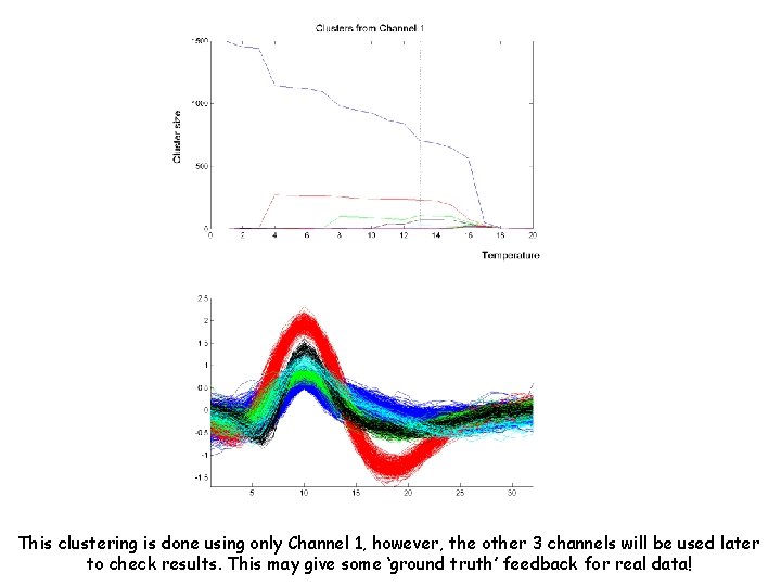
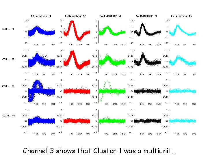
This clustering is done using only Channel 1, however, the other 3 channels will be used later to check results. This may give some ‘ground truth’ feedback for real data!

Channel 3 shows that Cluster 1 was a multiunit…

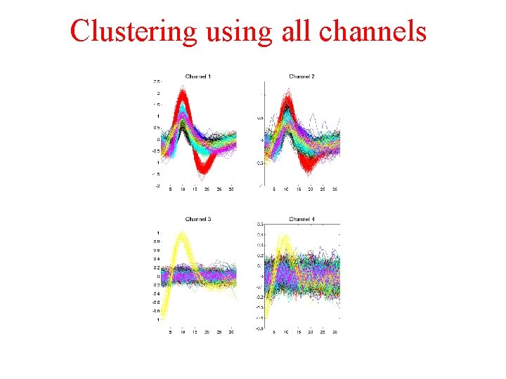
Clustering using all channels

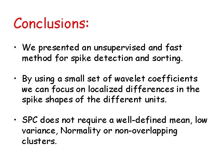
Conclusions: • We presented an unsupervised and fast method for spike detection and sorting. • By using a small set of wavelet coefficients we can focus on localized differences in the spike shapes of the different units. • SPC does not require a well-defined mean, low variance, Normality or non-overlapping clusters.